16.1 Introducing Graphs

contents ← prev up next →

16.1 Introducing Graphs

16.1.1 Understanding Graphs

16.1.2 Representations

16.1.2.1 Links by Name

16.1.2.2 Links by Indices

16.1.2.3 A List of Edges

16.1.2.4 Abstracting Representations

16.1.3 Measuring Complexity for Graphs

In From Acyclicity to Cycles we introduced a special kind of sharing: when the data become cyclic, i.e., there exist values such that traversing other reachable values from them eventually gets you back to the value at which you began. Data that have this characteristic are called graphs.Technically, a cycle is not necessary to be a graph; a tree or a DAG is also regarded as a (degenerate) graph. In this section, however, we are interested in graphs that have the potential for cycles.

Lots of very important data are graphs. For instance, the people and connections in social media form a graph: the people are nodes or vertices and the connections (such as friendships) are links or edges. They form a graph because for many people, if you follow their friends and then the friends of their friends, you will eventually get back to the person you started with. (Most simply, this happens when two people are each others’ friends.) The Web, similarly is a graph: the nodes are pages and the edges are links between pages. The Internet is a graph: the nodes are machines and the edges are links between machines. A transportation network is a graph: e.g., cities are nodes and the edges are transportation links between them. And so on. Therefore, it is essential to understand graphs to represent and process a great deal of interesting real-world data.

Graphs are important and interesting for not only practical but also principled reasons. The property that a traversal can end up where it began means that traditional methods of processing will no longer work: if it blindly processes every node it visits, it could end up in an infinite loop. Therefore, we need better structural recipes for our programs. In addition, graphs have a very rich structure, which lends itself to several interesting computations over them. We will study both these aspects of graphs below.

16.1.1 Understanding Graphs

Consider again the binary trees we saw earlier [Re-Examining Equality]. Let’s now try to distort the definition of a “tree” by creating ones with cycles, i.e., trees with nodes that point back to themselves (in the sense of identical). As we saw earlier [From Acyclicity to Cycles], it is not completely straightforward to create such a structure, but what we saw earlier [Streams From Functions] can help us here, by letting us suspend the evaluation of the cyclic link. That is, we have to not only use rec, we must also use a function to delay evaluation. In turn, we have to update the annotations on the fields. Since these are not going to be “trees” any more, we’ll use a name that is suggestive but not outright incorrect:

data BinT:
  | leaf
  | node(v, l :: ( -> BinT), r :: ( -> BinT))
end

Now let’s try to construct some cyclic values. Here are a few examples:

rec tr = node("rec", lam(): tr end, lam(): tr end)
t0 = node(0, lam(): leaf end, lam(): leaf end)
t1 = node(1, lam(): t0 end, lam(): t0 end)
t2 = node(2, lam(): t1 end, lam(): t1 end)

Now let’s try to compute the size of a BinT. Here’s the obvious program:

fun sizeinf(t :: BinT) -> Number:
  cases (BinT) t:
    | leaf => 0
    | node(v, l, r) =>
      ls = sizeinf(l())
      rs = sizeinf(r())
      1 + ls + rs
  end
end

(We’ll see why we call it sizeinf in a moment.)

Do Now!
What happens when we call sizeinf(tr)?

It goes into an infinite loop: hence the inf in its name.

There are two very different meanings for “size”. One is, “How many times can we traverse an edge?” The other is, “How many distinct nodes were constructed as part of the data structure?” With trees, by definition, these two are the same. With a DAG the former exceeds the latter but only by a finite amount. With a general graph, the former can exceed the latter by an infinite amount. In the case of a datum like tr, we can in fact traverse edges an infinite number of times. But the total number of constructed nodes is only one! Let’s write this as test cases in terms of a size function, to be defined:

check:
  size(tr) is 1
  size(t0) is 1
  size(t1) is 2
  size(t2) is 3
end

It’s clear that we need to somehow remember what nodes we have visited previously: that is, we need a computation with “memory”. In principle this is easy: we just create an extra data structure that checks whether a node has already been counted. As long as we update this data structure correctly, we should be all set. Here’s an implementation.

fun sizect(t :: BinT) -> Number:
  fun szacc(shadow t :: BinT, seen :: List<BinT>) -> Number:
    if has-id(seen, t):
      0
    else:
      cases (BinT) t:
        | leaf => 0
        | node(v, l, r) =>
          ns = link(t, seen)
          ls = szacc(l(), ns)
          rs = szacc(r(), ns)
          1 + ls + rs
      end
    end
  end
  szacc(t, empty)
end

The extra parameter, seen, is called an accumulator, because it “accumulates” the list of seen nodes.Note that this could just as well be a set; it doesn’t have to be a list. The support function it needs checks whether a given node has already been seen:

fun has-id<A>(seen :: List<A>, t :: A):
  cases (List) seen:
    | empty => false
    | link(f, r) =>
      if f <=> t: true
      else: has-id(r, t)
      end
  end
end

How does this do? Well, sizect(tr) is indeed 1, but sizect(t1) is 3 and sizect(t2) is 7!

Do Now!
Explain why these answers came out as they did.

The fundamental problem is that we’re not doing a very good job of remembering! Look at this pair of lines:

ls = szacc(l(), ns)
rs = szacc(r(), ns)

The nodes seen while traversing the left branch are effectively forgotten, because the only nodes we remember when traversing the right branch are those in ns: namely, the current node and those visited “higher up”. As a result, any nodes that “cross sides” are counted twice.

The remedy for this, therefore, is to remember every node we visit. Then, when we have no more nodes to process, instead of returning only the size, we should return all the nodes visited until now. This ensures that nodes that have multiple paths to them are visited on only one path, not more than once. The logic for this is to return two values from each traversal—the size and all the visited nodes—and not just one.

fun size(t :: BinT) -> Number:
  fun szacc(shadow t :: BinT, seen :: List<BinT>)
    -> {n :: Number, s :: List<BinT>}:
    if has-id(seen, t):
      {n: 0, s: seen}
    else:
      cases (BinT) t:
        | leaf => {n: 0, s: seen}
        | node(v, l, r) =>
          ns = link(t, seen)
          ls = szacc(l(), ns)
          rs = szacc(r(), ls.s)
          {n: 1 + ls.n + rs.n, s: rs.s}
      end
    end
  end
  szacc(t, empty).n
end

Sure enough, this function satisfies the above tests.

16.1.2 Representations

The representation we’ve seen above for graphs is certainly a start towards creating cyclic data, but it’s not very elegant. It’s both error-prone and inelegant to have to write lam everywhere, and remember to apply functions to () to obtain the actual values. Therefore, here we explore other representations of graphs that are more conventional and also much simpler to manipulate.

There are numerous ways to represent graphs, and the choice of representation depends on several factors:

The structure of the graph, and in particular, its density. We will discuss this further later [Measuring Complexity for Graphs].
The representation in which the data are provided by external sources. Sometimes it may be easier to simply adapt to their representation; in particular, in some cases there may not even be a choice.
The features provided by the programming language, which make some representations much harder to use than others.

In [Several Variations on Sets], we explore the idea of having many different representations for one datatype. As we will see, this is very true of graphs as well. Therefore, it would be best if we could arrive at a common interface to process graphs, so that all later programs can be written in terms of this interface, without overly depending on the underlying representation.

In terms of representations, there are three main things we need:

A way to construct graphs.
A way to identify (i.e., tell apart) nodes or vertices in a graph.
Given a way to identify nodes, a way to get that node’s neighbors in the graph.

Any interface that satisfies these properties will suffice. For simplicity, we will focus on the second and third of these and not abstract over the process of constructing a graph.

Our running example will be a graph whose nodes are cities in the United States and edges are direct flight connections between them:

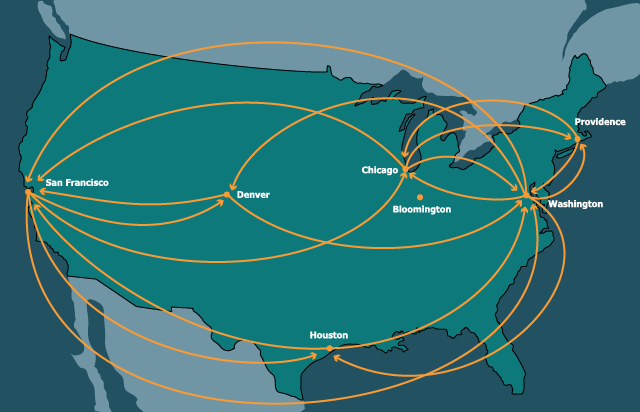
16.1.2.1 Links by Name

Here’s our first representation. We will assume that every node has a unique name (such a name, when used to look up information in a repository of data, is sometimes called a key). A node is then a key, some information about that node, and a list of keys that refer to other nodes:

type Key = String

data KeyedNode:
  | keyed-node(key :: Key, content, adj :: List<String>)
end

type KNGraph = List<KeyedNode>

type Node = KeyedNode
type Graph = KNGraph

(Here we’re assuming our keys are strings.)

Here’s a concrete instance of such a graph:The prefix kn- stands for “keyed node”.

kn-cities :: Graph = block:
  knWAS = keyed-node("was", "Washington", [list: "chi", "den", "saf", "hou", "pvd"])
  knORD = keyed-node("chi", "Chicago", [list: "was", "saf", "pvd"])
  knBLM = keyed-node("bmg", "Bloomington", [list: ])
  knHOU = keyed-node("hou", "Houston", [list: "was", "saf"])
  knDEN = keyed-node("den", "Denver", [list: "was", "saf"])
  knSFO = keyed-node("saf", "San Francisco", [list: "was", "den", "chi", "hou"])
  knPVD = keyed-node("pvd", "Providence", [list: "was", "chi"])
  [list: knWAS, knORD, knBLM, knHOU, knDEN, knSFO, knPVD]
end

Given a key, here’s how we look up its neighbor:

fun find-kn(key :: Key, graph :: Graph) -> Node:
  matches = for filter(n from graph):
    n.key == key
  end
  matches.first # there had better be exactly one!
end

Exercise
Convert the comment in the function into an invariant about the datum. Express this invariant as a refinement and add it to the declaration of graphs.

With this support, we can look up neighbors easily:

fun kn-neighbors(city :: Key,  graph :: Graph) -> List<Key>:
  city-node = find-kn(city, graph)
  city-node.adj
end

When it comes to testing, some tests are easy to write. Others, however, might require describing entire nodes, which can be unwieldy, so for the purpose of checking our implementation it suffices to examine just a part of the result:

check:
  ns = kn-neighbors("hou", kn-cities)

  ns is [list: "was", "saf"]

  map(_.content, map(find-kn(_, kn-cities), ns)) is
    [list: "Washington", "San Francisco"]
end

16.1.2.2 Links by Indices

In some languages, it is common to use numbers as names. This is especially useful when numbers can be used to get access to an element in a constant amount of time (in return for having a bound on the number of elements that can be accessed). Here, we use a list—which does not provide constant-time access to arbitrary elements—to illustrate this concept. Most of this will look very similar to what we had before; we’ll comment on a key difference at the end.

First, the datatype:The prefix ix- stands for “indexed”.

data IndexedNode:
  | idxed-node(content, adj :: List<Number>)
end

type IXGraph = List<IndexedNode>

type Node = IndexedNode
type Graph = IXGraph

Our graph now looks like this:

ix-cities :: Graph = block:
  inWAS = idxed-node("Washington", [list: 1, 4, 5, 3, 6])
  inORD = idxed-node("Chicago", [list: 0, 5, 6])
  inBLM = idxed-node("Bloomington", [list: ])
  inHOU = idxed-node("Houston", [list: 0, 5])
  inDEN = idxed-node("Denver", [list: 0, 5])
  inSFO = idxed-node("San Francisco", [list: 0, 4, 3])
  inPVD = idxed-node("Providence", [list: 0, 1])
  [list: inWAS, inORD, inBLM, inHOU, inDEN, inSFO, inPVD]
end

where we’re assuming indices begin at 0. To find a node:

fun find-ix(idx :: Key, graph :: Graph) -> Node:
  lists.get(graph, idx)
end

We can then find neighbors almost as before:

fun ix-neighbors(city :: Key,  graph :: Graph) -> List<Key>:
  city-node = find-ix(city, graph)
  city-node.adj
end

Finally, our tests also look similar:

check:
  ns = ix-neighbors(3, ix-cities)

  ns is [list: 0, 5]

  map(_.content, map(find-ix(_, ix-cities), ns)) is
    [list: "Washington", "San Francisco"]
end

Something deeper is going on here. The keyed nodes have intrinsic keys: the key is part of the datum itself. Thus, given just a node, we can determine its key. In contrast, the indexed nodes represent extrinsic keys: the keys are determined outside the datum, and in particular by the position in some other data structure. Given a node and not the entire graph, we cannot know for what its key is. Even given the entire graph, we can only determine its key by using identical, which is a rather unsatisfactory approach to recovering fundamental information. This highlights a weakness of using extrinsically keyed representations of information. (In return, extrinsically keyed representations are easier to reassemble into new collections of data, because there is no danger of keys clashing: there are no intrinsic keys to clash.)

16.1.2.3 A List of Edges

The representations we have seen until now have given priority to nodes, making edges simply a part of the information in a node. We could, instead, use a representation that makes edges primary, and nodes simply be the entities that lie at their ends:The prefix le- stands for “list of edges”.

data Edge:
  | edge(src :: String, dst :: String)
end

type LEGraph = List<Edge>

type Graph = LEGraph

Then, our flight network becomes:

le-cities :: Graph =
  [list:
    edge("Washington", "Chicago"),
    edge("Washington", "Denver"),
    edge("Washington", "San Francisco"),
    edge("Washington", "Houston"),
    edge("Washington", "Providence"),
    edge("Chicago", "Washington"),
    edge("Chicago", "San Francisco"),
    edge("Chicago", "Providence"),
    edge("Houston", "Washington"),
    edge("Houston", "San Francisco"),
    edge("Denver", "Washington"),
    edge("Denver", "San Francisco"),
    edge("San Francisco", "Washington"),
    edge("San Francisco", "Denver"),
    edge("San Francisco", "Houston"),
    edge("Providence", "Washington"),
    edge("Providence", "Chicago") ]

Observe that in this representation, nodes that are not connected to other nodes in the graph simply never show up! You’d therefore need an auxilliary data structure to keep track of all the nodes.

To obtain the set of neighbors:

fun le-neighbors(city :: Key, graph :: Graph) -> List<Key>:
  neighboring-edges = for filter(e from graph):
    city == e.src
  end
  names = for map(e from neighboring-edges): e.dst end
  names
end

And to be sure:

check:
  le-neighbors("Houston", le-cities) is
    [list: "Washington", "San Francisco"]
end

However, this representation makes it difficult to store complex information about a node without replicating it. Because nodes usually have rich information while the information about edges tends to be weaker, we often prefer node-centric representations. Of course, an alternative is to think of the node names as keys into some other data structure from which we can retrieve rich information about nodes.

16.1.2.4 Abstracting Representations

We would like a general representation that lets us abstract over the specific implementations. We will assume that broadly we have available a notion of Node that has content, a notion of Keys (whether or not intrinsic), and a way to obtain the neighbors—a list of keys—given a key and a graph. This is sufficient for what follows. However, we still need to choose concrete keys to write examples and tests. For simplicity, we’ll use string keys [Links by Name].

16.1.3 Measuring Complexity for Graphs

Before we begin to define algorithms over graphs, we should consider how to measure the size of a graph. A graph has two components: its nodes and its edges. Some algorithms are going to focus on nodes (e.g., visiting each of them), while others will focus on edges, and some will care about both. So which do we use as the basis for counting operations: nodes or edges?

It would help if we can reduce these two measures to one. To see whether that’s possible, suppose a graph has \(k\) nodes. Then its number of edges has a wide range, with these two extremes:

No two nodes are connected. Then there are no edges at all.
Every two nodes is connected. Then there are essentially as many edges as the number of pairs of nodes.

The number of nodes can thus be significantly less or even significantly more than the number of edges. Were this difference a matter of constants, we could have ignored it; but it’s not. As a graph tends towards the former extreme, the ratio of nodes to edges approaches \(k\) (or even exceeds it, in the odd case where there are no edges, but this graph is not very interesting); as it tends towards the latter, it is the ratio of edges to nodes that approaches \(k^2\). In other words, neither measure subsumes the other by a constant independent of the graph.

Therefore, when we want to speak of the complexity of algorithms over graphs, we have to consider the sizes of both the number of nodes and edges. In a connected graphA graph is connected if, from every node, we can traverse edges to get to every other node., however, there must be at least as many edges as nodes, which means the number of edges dominates the number of nodes. Since we are usually processing connected graphs, or connected parts of graphs one at a time, we can bound the number of nodes by the number of edges.

contents ← prev up next →

I	Introduction
II	Introduction to Programming
III	From Pyret to Python
IV	Programming With State
V	Algorithm Analysis
VI	Data Structures with Analysis
VII	Advanced Topics
VIII	Interactive Programs
IX	Appendices

16.1	Introducing Graphs
16.2	Basic Graph Traversals
16.3	Graphs With Weighted Edges
16.4	Shortest (or Lightest) Paths
16.5	Moravian Spanning Trees

15	Directed Acyclic Graphs
16	Graphs
17	Several Variations on Sets

16.1.1	Understanding Graphs
16.1.2	Representations
16.1.3	Measuring Complexity for Graphs