21 Avoiding Recomputation by Remembering Answers
We have on several instances already referred to a ☛ space-time tradeoff. The most obvious tradeoff is when a computation “remembers” prior results and, instead of recomputing them, looks them up and returns the answers. This is an instance of the tradeoff because it uses space (to remember prior answers) in place of time (recomputing the answer). Let’s see how we can write such computations.
21.1 An Interesting Numeric Sequence
Suppose we want to create properly-parenthesized expressions, and ignore all non-parenthetical symbols. How many ways are there of creating parenthesized expressions given a certain number of opening (equivalently, closing) parentheses?
If we have zero opening parentheses, the only expression we can create is the empty expression. If we have one opening parenthesis, the only one we can construct is “()” (there must be a closing parenthesis since we’re interested only in properly-parenthesized expressions). If we have two opening parentheses, we can construct “(())” and “()()”. Given three, we can construct “((()))”, “(())()”, “()(())”, “()()()”, and “(()())”, for a total of five. And so on. Observe that the solutions at each level use all the possible solutions at one level lower, combined in all the possible ways.
fun catalan(n):
  if n == 0: 1
  else if n > 0:
    for fold(acc from 0, k from range(0, n)):
      acc + (catalan(k) * catalan(n - 1 - k))
    end
  end
endcheck:
catalan(0) is 1
catalan(1) is 1
catalan(2) is 2
catalan(3) is 5
catalan(4) is 14
catalan(5) is 42
catalan(6) is 132
catalan(7) is 429
catalan(8) is 1430
catalan(9) is 4862
catalan(10) is 16796
catalan(11) is 58786
end10 and 20—Do Now!
Check at what value you start to observe a significant slowdown on your machine. Plot the graph of running time against input size. What does this suggest?
The reason the Catalan computation takes so long is precisely because of what we alluded to earlier: at each level, we depend on computing the Catalan number of all the smaller levels; this computation in turn needs the numbers of all of its smaller levels; and so on down the road.
Exercise
Map the subcomputations of
catalanto see why the computation time explodes as it does. What is the worst-case time complexity of this function?
Here is a graphical representation of all the sub-computations the
Catalan function does for input 3:
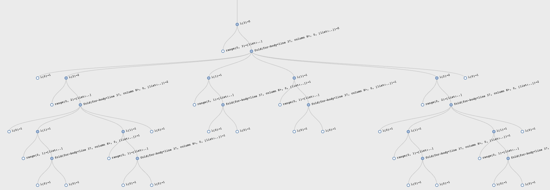
Observe the very symmetric computation, reflecting the formula.
21.1.1 Using State to Remember Past Answers
Therefore, this is clearly a case where trading space for time is likely to be of help. How do we do this? We need a notion of memory that records all previous answers and, on subsequent attempts to compute them, checks whether they are already known and, if so, just returns them instead of recomputing them.
Do Now!
What critical assumption is this based on?
Naturally, this assumes that for a given input, the answer will
always be the same. As we have seen, functions with state violate
this liberally, so typical stateful functions cannot utilize this
optimization. Ironically, we will use state to implement this
optimization, so we will have a stateful function that always returns
the same answer on a given input—
data MemoryCell:
  | mem(in, out)
end

var memory :: List<MemoryCell> = emptycatalan need to change? We have to first look for
whether the value is already in memory; if it is, we return it
without any further computation, but if it isn’t, then we compute the
result, store it in memory, and then return it:
fun catalan(n :: Number) -> Number:
  answer = find(lam(elt): elt.in == n end, memory)
  cases (Option) answer block:
    | none =>
      result =
        if n == 0: 1
        else if n > 0:
          for fold(acc from 0, k from range(0, n)):
            acc + (catalan(k) * catalan(n - 1 - k))
          end
        end
      memory := link(mem(n, result), memory)
      result
    | some(v) => v.out
  end
endcatalan(50).Do Now!
Trace through a call of this revised function and see how many calls it makes.
Here is a revised visualization of computing for input 3:
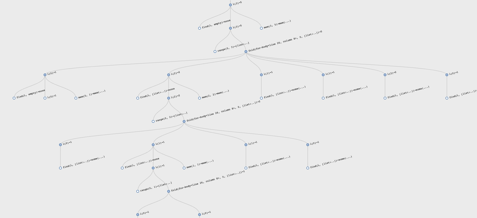
Observe the asymmetric computation: the early calls perform the computations, while the latter calls simply look up the results.
This process, of converting a function into a version that remembers its past answers, is called memoization.
21.1.2 From a Tree of Computation to a DAG
What we have subtly done is to convert a tree of computation into a
DAG over the same computation, with equivalent calls being
reused. Whereas previously each call was generating lots of recursive
calls, which induced still more recursive calls, now we are reusing
previous recursive calls—
This has an important complexity benefit. Whereas previously we were
performing a super-exponential number of calls, now we perform only
one call per input and share all previous calls—catalan(n) to take a number of fresh calls proportional to
n. Looking up the result of a previous call takes time
proportional to the size of memory (because we’ve represented
it as a list; better representations would improve on that), but that
only contributes another linear multiplicative factor, reducing the
overall complexity to quadratic in the size of the input. This is a
dramatic reduction in overall complexity. In contrast, other uses of
memoization may result in much less dramatic improvements, turning the
use of this technique into a true engineering trade-off.
21.1.3 The Complexity of Numbers
As we start to run larger computations, however, we may start to
notice that our computations are starting to take longer than linear
growth. This is because our numbers are growing arbitrarily
large—catalan(100) is
896519947090131496687170070074100632420837521538745909320—
21.1.4 Abstracting Memoization
Now we’ve achieved the desired complexity improvement, but there is
still something unsatisfactory about the structure of our revised
definition of catalan: the act of memoization is deeply
intertwined with the definition of a Catalan number, even though these
should be intellectually distinct. Let’s do that next.
In effect, we want to separate our program into two parts. One part
defines a general notion of memoization, while the other defines
catalan in terms of this general notion.
data MemoryCell:
  | mem(in, out)
end

fun memoize-1<T, U>(f :: (T -> U)) -> (T -> U):

  var memory :: List<MemoryCell> = empty

  lam(n):
    answer = find(lam(elt): elt.in == n end, memory)
    cases (Option) answer block:
      | none =>
        result = f(n)
        memory := link(mem(n, result), memory)
        result
      | some(v) => v.out
    end
  end
endmemoize-1 to indicate that this is a
memoizer for single-argument functions. Observe that the code
above is virtually identical to what we had before, except where we
had the logic of Catalan number computation, we now have the parameter
f determining what to do.catalan as follows:
rec catalan :: (Number -> Number) =
  memoize-1(
    lam(n):
      if n == 0: 1
      else if n > 0:
        for fold(acc from 0, k from range(0, n)):
          acc + (catalan(k) * catalan(n - 1 - k))
        end
      end
end)We don’t write
fun catalan(...): ...;because the procedure bound tocatalanis produced bymemoize-1.Note carefully that the recursive calls to
catalanhave to be to the function bound to the result of memoization, thereby behaving like an object. Failing to refer to this same shared procedure means the recursive calls will not be memoized, thereby losing the benefit of this process.We need to use
recfor reasons we saw earlier [Streams From Functions].Each invocation of
memoize-1creates a new table of stored results. Therefore the memoization of different functions will each get their own tables rather than sharing tables, which is a bad idea!
Exercise
Why is sharing memoization tables a bad idea? Be concrete.
21.2 Edit-Distance for Spelling Correction
Text editors, word processors, mobile phones, and various other devices now routinely implement spelling correction or offer suggestions on (mis-)spellings. How do they do this? Doing so requires two capabilities: computing the distance between words, and finding words that are nearby according to this metric. In this section we will study the first of these questions. (For the purposes of this discussion, we will not dwell on the exact definition of what a “word” is, and just deal with strings instead. A real system would need to focus on this definition in considerable detail.)
Do Now!
Think about how you might define the “distance between two words”. Does it define a metric space?
Exercise
Will the definition we give below define a metric space over the set of words?
That the distance from a word to itself be zero.
That the distance from a word to any word other than itself be strictly positive. (Otherwise, given a word that is already in the dictionary, the “correction” might be a different dictionary word.)
That the distance between two words be symmetric, i.e., it shouldn’t matter in which order we pass arguments.
Exercise
Observe that we have not included the triangle inequality relative to the properties of a metric. Why not? If we don’t need the triangle inequality, does this let us define more interesting distance functions that are not metrics?
we left out a character;
we typed a character twice; or,
we typed one character when we meant another.
There are several variations of this definition possible. For now, we will consider the simplest one, which assumes that each of these errors has equal cost. For certain input devices, we may want to assign different costs to these mistakes; we might also assign different costs depending on what wrong character was typed (two characters adjacent on a keyboard are much more likely to be a legitimate error than two that are far apart). We will return briefly to some of these considerations later [Nature as a Fat-Fingered Typist].
check:
  levenshtein(empty, empty) is 0
  levenshtein([list: "x"], [list: "x"]) is 0
  levenshtein([list: "x"], [list: "y"]) is 1
  # one of about 600
  levenshtein(
    [list: "b", "r", "i", "t", "n", "e", "y"],
    [list: "b", "r", "i", "t", "t", "a", "n", "y"])
    is 3
  # http://en.wikipedia.org/wiki/Levenshtein_distance
  levenshtein(
    [list: "k", "i", "t", "t", "e", "n"],
    [list: "s", "i", "t", "t", "i", "n", "g"])
    is 3
  levenshtein(
    [list: "k", "i", "t", "t", "e", "n"],
    [list: "k", "i", "t", "t", "e", "n"])
    is 0
  # http://en.wikipedia.org/wiki/Levenshtein_distance
  levenshtein(
    [list: "S", "u", "n", "d", "a", "y"],
    [list: "S", "a", "t", "u", "r", "d", "a", "y"])
    is 3
  # http://www.merriampark.com/ld.htm
  levenshtein(
    [list: "g", "u", "m", "b", "o"],
    [list: "g", "a", "m", "b", "o", "l"])
    is 2
  # http://www.csse.monash.edu.au/~lloyd/tildeStrings/Alignment/92.IPL.html
  levenshtein(
    [list: "a", "c", "g", "t", "a", "c", "g", "t", "a", "c", "g", "t"],
    [list: "a", "c", "a", "t", "a", "c", "t", "t", "g", "t", "a", "c", "t"])
    is 4
  levenshtein(
    [list: "s", "u", "p", "e", "r", "c", "a", "l", "i",
      "f", "r", "a", "g", "i", "l", "i", "s", "t" ],
    [list: "s", "u", "p", "e", "r", "c", "a", "l", "y",
      "f", "r", "a", "g", "i", "l", "e", "s", "t" ])
    is 2
endrec levenshtein :: (List<String>, List<String> -> Number) =
<levenshtein-body>if is-empty(s) and is-empty(t): 0else if is-empty(s): t.length()
else if is-empty(t): s.length()else:
if s.first == t.first:
levenshtein(s.rest, t.rest)
else:
min3(
1 + levenshtein(s.rest, t),
1 + levenshtein(s, t.rest),
1 + levenshtein(s.rest, t.rest))
end
ends has one too many characters, so
we compute the cost as if we’re deleting it and finding the lowest
cost for the rest of the strings (but charging one for this deletion);
in the second case, we symmetrically assume t has one too many;
and in the third case, we assume one character got replaced by
another, so we charge one but consider the rest of both words (e.g.,
assume “s” was typed for “k” and continue with “itten” and
“itting”). This uses the following helper function:
fun min3(a :: Number, b :: Number, c :: Number):
num-min(a, num-min(b, c))
endThis algorithm will indeed pass all the tests we have written above, but with a problem: the running time grows exponentially. That is because, each time we find a mismatch, we recur on three subproblems. In principle, therefore, the algorithm takes time proportional to three to the power of the length of the shorter word. In practice, any prefix that matches causes no branching, so it is mismatches that incur branching (thus, confirming that the distance of a word with itself is zero only takes time linear in the size of the word).
Observe, however, that many of these subproblems are the same. For instance, given “kitten” and “sitting”, the mismatch on the initial character will cause the algorithm to compute the distance of “itten” from “itting” but also “itten” from “sitting” and “kitten” from “itting”. Those latter two distance computations will also involve matching “itten” against “itting”. Thus, again, we want the computation tree to turn into a DAG of expressions that are actually evaluated.
data MemoryCell2<T, U, V>:
| mem(in-1 :: T, in-2 :: U, out :: V)
end
fun memoize-2<T, U, V>(f :: (T, U -> V)) -> (T, U -> V):
var memory :: List<MemoryCell2<T, U, V>> = empty
lam(p, q):
answer = find(
lam(elt): (elt.in-1 == p) and (elt.in-2 == q) end,
memory)
cases (Option) answer block:
| none =>
result = f(p, q)
memory :=
link(mem(p, q, result), memory)
result
| some(v) => v.out
end
end
endlevenshtein to use memoization:
rec levenshtein :: (List<String>, List<String> -> Number) =
memoize-2(
lam(s, t):
if is-empty(s) and is-empty(t): 0
else if is-empty(s): t.length()
else if is-empty(t): s.length()
else:
  if s.first == t.first:
    levenshtein(s.rest, t.rest)
  else:
    min3(
      1 + levenshtein(s.rest, t),
      1 + levenshtein(s, t.rest),
      1 + levenshtein(s.rest, t.rest))
  end
end
end)memoize-2 is precisely what we saw
earlier as <levenshtein-body> (and now you know why we
defined levenshtein slightly oddly, not using fun).The complexity of this algorithm is still non-trivial. First, let’s introduce the term suffix: the suffix of a string is the rest of the string starting from any point in the string. (Thus “kitten”, “itten”, “ten”, “n”, and “” are all suffixes of “kitten”.) Now, observe that in the worst case, starting with every suffix in the first word, we may need to perform a comparison against every suffix in the second word. Fortunately, for each of these suffixes we perform a constant computation relative to the recursion. Therefore, the overall time complexity of computing the distance between strings of length \(m\) and \(n\) is \(O([m, n \rightarrow m \cdot n])\). (We will return to space consumption later [Contrasting Memoization and Dynamic Programming].)
Exercise
Modify the above algorithm to produce an actual (optimal) sequence of edit operations. This is sometimes known as the traceback.
21.3 Nature as a Fat-Fingered Typist
We have talked about how to address mistakes made by humans. However, humans are not the only bad typists: nature is one, too!
When studying living matter we obtain sequences of amino acids and
other such chemicals that comprise molecules, such as DNA, that hold
important and potentially determinative information about the
organism. These sequences consist of similar fragments that we wish to
identify because they represent relationships in
the organism’s behavior or evolution.This section may
need to be skipped in
some states and countries.
Unfortunately, these sequences are never identical: like all
low-level programmers, nature slips up and sometimes makes mistakes in
copying (called—
The only difference between traditional presentations of Levenshtein and Smith-Waterman is something we alluded to earlier: why is every edit given a distance of one? Instead, in the Smith-Waterman presentation, we assume that we have a function that gives us the gap score, i.e., the value to assign every character’s alignment, i.e., scores for both matches and edits, with scores driven by biological considerations. Of course, as we have already noted, this need is not peculiar to biology; we could just as well use a “gap score” to reflect the likelihood of a substitution based on keyboard characteristics.
21.4 Dynamic Programming
We have used memoization as our canonical means of saving the values of past computations to reuse later. There is another popular technique for doing this called dynamic programming. This technique is closely related to memoization; indeed, it can be viewed as the dual method for achieving the same end. First we will see dynamic programming at work, then discuss how it differs from memoization.
Dynamic programming also proceeds by building up a memory of answers, and looking them up instead of recomputing them. As such, it too is a process for turning a computation’s shape from a tree to a DAG of actual calls. The key difference is that instead of starting with the largest computation and recurring to smaller ones, it starts with the smallest computations and builds outward to larger ones.
We will revisit our previous examples in light of this approach.
21.4.1 Catalan Numbers with Dynamic Programming
MAX-CAT = 11

answers :: Array<Option<Number>> = array-of(none, MAX-CAT + 1)catalan function simply looks up the answer in this
array:
fun catalan(n):
  cases (Option) array-get-now(answers, n):
    | none => raise("looking at uninitialized value")
    | some(v) => v
  end
endblock:
fun fill-catalan(upper) block:
  array-set-now(answers, 0, some(1))
  when upper > 0:
    for each(n from range(1, upper + 1)):
      block:
        cat-at-n =
          for fold(acc from 0, k from range(0, n)):
            acc + (catalan(k) * catalan(n - 1 - k))
          end
        array-set-now(answers, n, some(cat-at-n))
      end
    end
  end
end

fill-catalan(MAX-CAT)Notice that we have had to undo the natural recursive
definition—catalan to some value, that index of answers will have
not yet been initialized, resultingin an error. In fact, however, we
know that because we fill all smaller indices in answers before
computing the next larger one, we will never actually encounter this
error. Note that this requires careful reasoning about our program,
which we did not need to perform when using memoization because
there we made precisely the recursive call we needed, which either
looked up the value or computed it afresh.
21.4.2 Levenshtein Distance and Dynamic Programming
fun levenshtein(s1 :: List<String>, s2 :: List<String>) block:
  <levenshtein-dp/1>
ends1 and as many columns as the length of
s2. At each position, we will record the edit distance for the
prefixes of s1 and s2 up to the indices represented by
that position in the table.s1-len = s1.length()
s2-len = s2.length()
answers = array2d(s1-len + 1, s2-len + 1, none)
<levenshtein-dp/2>answers inside levenshtein, we
can determine the exact size it needs to be based on the inputs,
rather than having to over-allocate or dynamically grow the array.Exercise
Define the functionsarray2d :: Number, Number, A -> Array<A> set-answer :: Array<A>, Number, Number, A -> Nothing get-answer :: Array<A>, Number, Number -> A
none, so we will get an
error if we accidentally try to use an uninitialized
entry.Which proved to be necessary when
writing and debugging this code! It will
therefore be convenient to create helper functions that let us
pretend the table contains only numbers:
fun put(s1-idx :: Number, s2-idx :: Number, n :: Number):
  set-answer(answers, s1-idx, s2-idx, some(n))
end
fun lookup(s1-idx :: Number, s2-idx :: Number) -> Number block:
  a = get-answer(answers, s1-idx, s2-idx)
  cases (Option) a:
    | none => raise("looking at uninitialized value")
    | some(v) => v
  end
ends2 is empty, and the
column where s1 is empty. At \((0, 0)\), the edit distance is
zero; at every position thereafter, it is the distance of that
position from zero, because that many characters must be added to one
or deleted from the other word for the two to coincide:
for each(s1i from range(0, s1-len + 1)):
  put(s1i, 0, s1i)
end
for each(s2i from range(0, s2-len + 1)):
  put(0, s2i, s2i)
end
<levenshtein-dp/4>0 to s1-len - 1 and s2-len - 1, which are
precisely the ranges of values produced by range(0, s1-len) and
range(0, s2-len).
for each(s1i from range(0, s1-len)):
  for each(s2i from range(0, s2-len)):
  <levenshtein-dp/compute-dist>
  end
end
<levenshtein-dp/get-result>Do Now!
Is this strictly true?
No, it isn’t. We did first fill in values for the “borders” of the table. This is because doing so in the midst of <levenshtein-dp/compute-dist> would be much more annoying. By initializing all the known values, we keep the core computation cleaner. But it does mean the order in which we fill in the table is fairly complex.
dist =
  if get(s1, s1i) == get(s2, s2i):
    lookup(s1i, s2i)
  else:
    min3(
      1 + lookup(s1i, s2i + 1),
      1 + lookup(s1i + 1, s2i),
      1 + lookup(s1i, s2i))
  end
put(s1i + 1, s2i + 1, dist)-1 so that the main computation looks
traditional.lookup(s1-len, s2-len)fun levenshtein(s1 :: List<String>, s2 :: List<String>) block:
s1-len = s1.length()
s2-len = s2.length()
answers = array2d(s1-len + 1, s2-len + 1, none)
fun put(s1-idx :: Number, s2-idx :: Number, n :: Number):
set-answer(answers, s1-idx, s2-idx, some(n))
end
fun lookup(s1-idx :: Number, s2-idx :: Number) -> Number block:
a = get-answer(answers, s1-idx, s2-idx)
cases (Option) a:
| none => raise("looking at uninitialized value")
| some(v) => v
end
end
for each(s1i from range(0, s1-len + 1)):
put(s1i, 0, s1i)
end
for each(s2i from range(0, s2-len + 1)):
put(0, s2i, s2i)
end
for each(s1i from range(0, s1-len)):
for each(s2i from range(0, s2-len)):
dist =
if get(s1, s1i) == get(s2, s2i):
lookup(s1i, s2i)
else:
min3(
1 + lookup(s1i, s2i + 1),
1 + lookup(s1i + 1, s2i),
1 + lookup(s1i, s2i))
end
put(s1i + 1, s2i + 1, dist)
end
end
lookup(s1-len, s2-len)
end21.5 Contrasting Memoization and Dynamic Programming
Now that we’ve seen two very different techniques for avoiding recomputation, it’s worth contrasting them. The important thing to note is that memoization is a much simpler technique: write the natural recursive definition; determine its time complexity; decide whether this is problematic enough to warrant a space-time trade-off; and if it is, apply memoization. The code remains clean, and subsequent readers and maintainers will be grateful for that. In contrast, dynamic programming requires a reorganization of the algorithm to work bottom-up, which can often make the code harder to follow and full of subtle invariants about boundary conditions and computation order.
That said, the dynamic programming solution can sometimes be more computationally efficient. For instance, in the Levenshtein case, observe that at each table element, we (at most) only ever use the ones that are from the previous row and column. That means we never need to store the entire table; we can retain just the fringe of the table, which reduces space to being proportional to the sum, rather than product, of the length of the words. In a computational biology setting (when using Smith-Waterman), for instance, this saving can be substantial. This optimization is essentially impossible for memoization.
Memoization |
| Dynamic Programming |
Top-down |
| Bottom-up |
Depth-first |
| Breadth-first |
Black-box |
| Requires code reorganization |
All stored calls are necessary |
| May do unnecessary computation |
Cannot easily get rid of unnecessary data |
| Can more easily get rid of unnecessary data |
Can never accidentally use an uninitialized answer |
| Can accidentally use an uninitialized answer |
Needs to check for the presence of an answer |
| Can be designed to not need to check for the presence of an answer |
From a software design perspective, there are two more considerations.
First, the performance of a memoized solution can trail that of dynamic programming when the memoized solution uses a generic data structure to store the memo table, whereas a dynamic programming solution will invariably use a custom data structure (since the code needs to be rewritten against it anyway). Therefore, before switching to dynamic programming for performance reasons, it makes sense to try to create a custom memoizer for the problem: the same knowledge embodied in the dynamic programming version can often be encoded in this custom memoizer (e.g., using an array instead of list to improve access times). This way, the program can enjoy speed comparable to that of dynamic programming while retaining readability and maintainability.
Second, suppose space is an important consideration and the dynamic programming version can make use of significantly less space. Then it does make sense to employ dynamic programming instead. Does this mean the memoized version is useless?
Do Now!
What do you think? Do we still have use for the memoized version?
Yes, of course we do! It can serve as an oracle [Oracles for Testing] for the dynamic
programming version, since the two are supposed to produce identical
answers anyway—
In short, always first produce the memoized version. If you need more performance, consider customizing the memoizer’s data structure. If you need to also save space, and can arrive at a more space-efficient dynamic programming solution, then keep both versions around, using the former to test the latter (the person who inherits your code and needs to alter it will thank you!).
Exercise
We have characterized the fundamental difference between memoization and dynamic programming as that between top-down, depth-first and bottom-up, breadth-first computation. This should naturally raise the question, what about:
top-down, breadth-first
bottom-up, depth-first
orders of computation. Do they also have special names that we just happen to not know? Are they uninteresting? Or do they not get discussed for a reason?