III Algorithms
18 Predicting Growth
18.5 The Tabular Method for Singly-Structurally-Recursive Functions |
We will now commence the study of determining how long a computation takes. We’ll begin with a little (true) story.
18.1 A Little (True) Story
My student Debbie recently wrote tools to analyze data for a startup. The company collects information about product scans made on mobile phones, and Debbie’s analytic tools classified these by product, by region, by time, and so on. As a good programmer, Debbie first wrote synthetic test cases, then developed her programs and tested them. She then obtained some actual test data from the company, broke them down into small chunks, computed the expected answers by hand, and tested her programs again against these real (but small) data sets. At the end of this she was ready to declare the programs ready.
The company was rightly reluctant to share the entire dataset with outsiders, and in turn we didn’t want to be responsible for carefully guarding all their data.
Even if we did get a sample of their data, as more users used their product, the amount of data they had was sure to grow.
Debbie was given 100,000 data points. She broke them down into input sets of 10, 100, 1,000, 10,000, and 100,000 data points, ran her tools on each input size, and plotted the result.
From this graph we have a good bet at guessing how long the tool would take on a dataset of 50,000. It’s much harder, however, to be sure how long it would take on datasets of size 1.5 million or 3 million or 10 million.These processes are respectively called interpolation and extrapolation. We’ve already explained why we couldn’t get more data from the company. So what could we do?
As another problem, suppose we have multiple implementations available. When we plot their running time, say the graphs look like this, with red, green, and blue each representing different implementations. On small inputs, suppose the running times look like this:
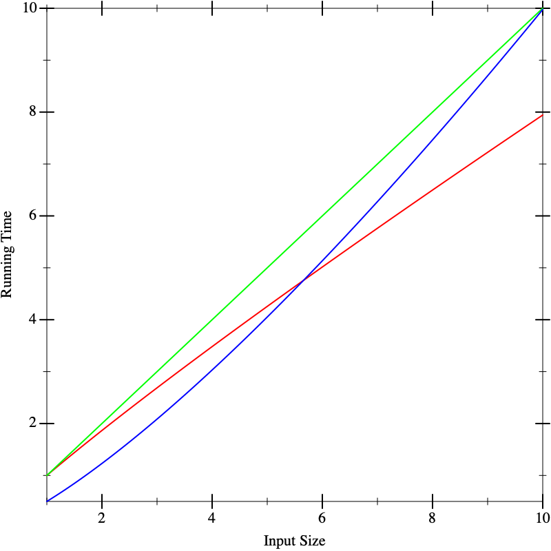
This doesn’t seem to help us distinguish between the implementations. Now suppose we run the algorithms on larger inputs, and we get the following graphs:
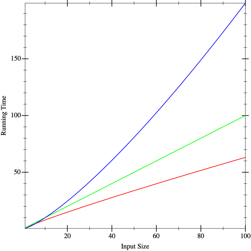
Now we seem to have a clear winner (red), though it’s not clear there is much to give between the other two (blue and green). But if we calculate on even larger inputs, we start to see dramatic differences:
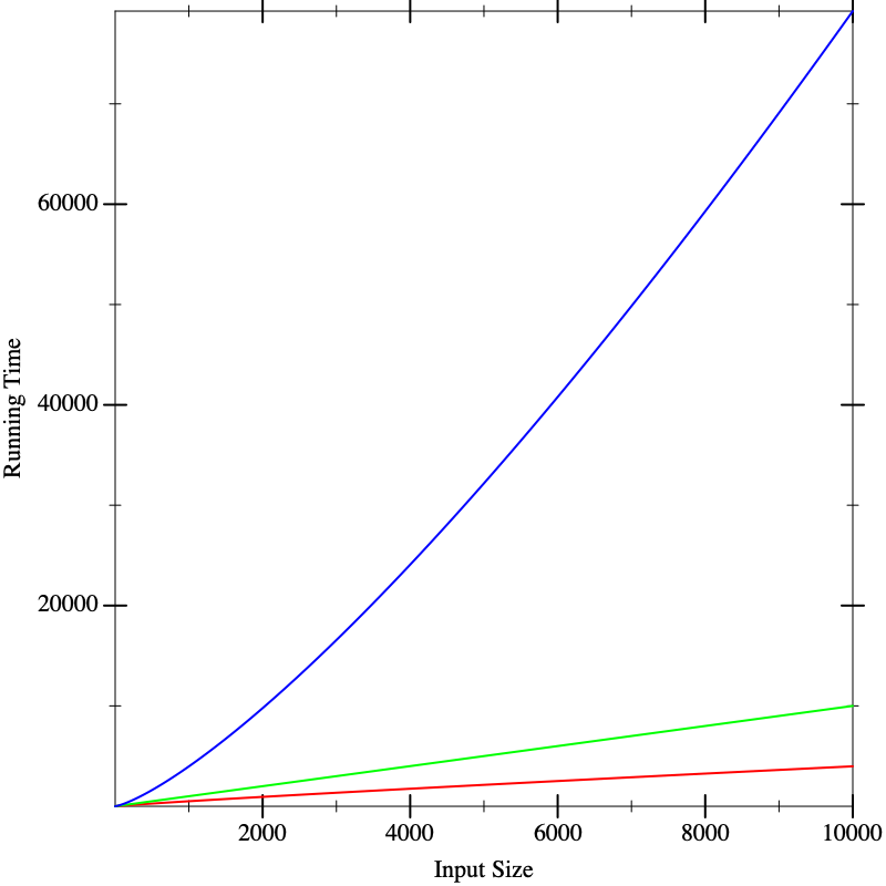
In fact, the functions that resulted in these lines were the same in all three figures. What these pictures tell us is that it is dangerous to extrapolate too much from the performance on small inputs. If we could obtain closed-form descriptions of the performance of computations, it would be nice if we could compare them better. That is what we will do in the next section.
Responsible Computing: Choose Analysis Artifacts Wisely
As more and more decisions are guided by statistical analyses of data (performed by humans), it’s critical to recognize that data can be a poor proxy for the actual phenomenon that we seek to understand. Here, Debbie had data about program behavior, which led to mis-interpretations regarding which program is best. But Debbie also had the programs themselves, from which the data were generated. Analyzing the programs, rather than the data, is a more direct approach to assessing the performance of a program.
While the rest of this chapter is about analyzing programs as written in code, this point carries over to non-programs as well. You might want to understand the effectiveness of a process for triaging patients at a hospital, for example. In that case, you have both the policy documents (rules which may or may not have been turned into a software program to support managing patients) and data on the effectiveness of using that process. Responsible computing tells us to analyze both the process and its behavioral data, against knowledge about best practices in patient care, to evaluate the effectiveness of systems.
18.2 The Analytical Idea
With many physical processes, the best we can do is obtain as many data points as possible, extrapolate, and apply statistics to reason about the most likely outcome. Sometimes we can do that in computer science, too, but fortunately we computer scientists have an enormous advantage over most other sciences: instead of measuring a black-box process, we have full access to its internals, namely the source code. This enables us to apply analytical methods.“Analytical” means applying algebraic and other mathematical methods to make predictive statements about a process without running it. The answer we compute this way is complementary to what we obtain from the above experimental analysis, and in practice we will usually want to use a combination of the two to arrive a strong understanding of the program’s behavior.
The analytical idea is startlingly simple. We look at the source of the program and list the operations it performs. For each operation, we look up what it costs.We are going to focus on one kind of cost, namely running time. There are many other other kinds of costs one can compute. We might naturally be interested in space (memory) consumed, which tells us how big a machine we need to buy. We might also care about power, this tells us the cost of our energy bills, or of bandwidth, which tells us what kind of Internet connection we will need. In general, then, we’re interested in resource consumption. In short, don’t make the mistake of equating “performance” with “speed”: the costs that matter depend on the context in which the application runs. We add up these costs for all the operations. This gives us a total cost for the program.
Naturally, for most programs the answer will not be a constant number. Rather, it will depend on factors such as the size of the input. Therefore, our answer is likely to be an expression in terms of parameters (such as the input’s size). In other words, our answer will be a function.
There are many functions that can describe the running-time of a function. Often we want an upper bound on the running time: i.e., the actual number of operations will always be no more than what the function predicts. This tells us the maximum resource we will need to allocate. Another function may present a lower bound, which tells us the least resource we need. Sometimes we want an average-case analysis. And so on. In this text we will focus on upper-bounds, but keep in mind that all these other analyses are also extremely valuable.
Exercise
It is incorrect to speak of “the” upper-bound function, because there isn’t just one. Given one upper-bound function, can you construct another one?
18.3 A Cost Model for Pyret Running Time
We begin by presenting a cost model for the running time of Pyret programs. We are interested in the cost of running a program, which is tantamount to studying the expressions of a program. Simply making a definition does not cost anything; the cost is incurred only when we use a definition.
We will use a very simple (but sufficiently accurate) cost model:
every operation costs one unit of time in addition to the time needed
to evaluate its sub-expressions. Thus it takes one unit of time to
look up a variable or to allocate a constant. Applying primitive
functions also costs one unit of time. Everything else is a compound
expression with sub-expressions. The cost of a compound expression is
one plus that of each of its sub-expressions. For instance, the
running time cost of the expression e1 + e2 (for some
sub-expressions e1 and e2) is the running time for
e1 + the running time for e2 + 1. Thus the expression
17 + 29 has a cost of 3 (one for each sub-expression and one
for the addition); the expression 1 + (7 * (2 / 9)) costs 7.
First, we are using an abstract rather than concrete notion of time. This is unhelpful in terms of estimating the so-called “wall clock” running time of a program, but then again, that number depends on numerous factors—
not just what kind of processor and how much memory you have, but even what other tasks are running on your computer at the same time. In contrast, abstract time units are more portable. Second, not every operation takes the same number of machine cycles, whereas we have charged all of them the same number of abstract time units. As long as the actual number of cycles each one takes is bounded by a constant factor of the number taken by another, this will not pose any mathematical problems for reasons we will soon understand [Comparing Functions].
There is one especially tricky kind of expression: if (and its fancier
cousins, like cases and ask). How do we think about the cost of
an if? It always evaluates the condition. After that, it evaluates only
one of its branches. But we are interested in the worst case time,
i.e., what is the longest it could take? For a conditional, it’s the cost of
the condition added to the cost of the maximum of the two
branches.
18.4 The Size of the Input
We
gloss over the size of a number, treating it as constant. Observe that
the value of a number is exponentially larger than its
size: \(n\) digits in base \(b\) can represent \(b^n\) numbers.
Though irrelevant here,
when numbers are central—
It can be subtle to define the size of the argument. Suppose a
function consumes a list of numbers; it would be natural to define the
size of its argument to be the length of the list, i.e., the number of
links in the list. We could also define it to be twice as
large, to account for both the links and the individual
numbers (but as we’ll see [Comparing Functions], constants usually don’t matter).
But suppose a function consumes a list of music albums, and each music
album is itself a list of songs, each of which has information about
singers and so on. Then how we measure the size depends on what part
of the input the function being analyzed actually examines. If, say,
it only returns the length of the list of albums, then it is
indifferent to what each list element contains [Monomorphic Lists and Polymorphic Types],
and only the length of the list of albums matters. If, however, the
function returns a list of all the singers on every album, then it
traverses all the way down to individual songs, and we have to account
for all these data. In short, we care about the size of the
data potentially accessed by the function.
18.5 The Tabular Method for Singly-Structurally-Recursive Functions
Given sizes for the arguments, we simply examine the body of the function and add up the costs of the individual operations. Most interesting functions are, however, conditionally defined, and may even recur. Here we will assume there is only one structural recursive call. We will get to more general cases in a bit [Creating Recurrences].
When we have a function with only one recursive call, and it’s structural, there’s a handy technique we can use to handle conditionals.This idea is due to Prabhakar Ragde. We will set up a table. It won’t surprise you to hear that the table will have as many rows as the cond has clauses. But instead of two columns, it has seven! This sounds daunting, but you’ll soon see where they come from and why they’re there.
|Q|: the number of operations in the question
#Q: the number of times the question will execute
TotQ: the total cost of the question (multiply the previous two)
|A|: the number of operations in the answer
#A: the number of times the answer will execute
TotA: the total cost of the answer (multiply the previous two)
Total: add the two totals to obtain an answer for the clause
cond expression is obtained by
summing the Total column in the individual rows.In the process of computing these costs, we may come across recursive calls in an answer expression. So long as there is only one recursive call in the entire answer, ignore it.
Exercise
Once you’ve read the material on Creating Recurrences, come back to this and justify why it is okay to just skip the recursive call. Explain in the context of the overall tabular method.
Exercise
Excluding the treatment of recursion, justify (a) that these columns are individually accurate (e.g., the use of additions and multiplications is appropriate), and (b) sufficient (i.e., combined, they account for all operations that will be performed by that
condclause).
len function, noting before we
proceed that it does meet the criterion of having a single recursive
call where the argument is structural:
fun len(l):
  cases (List) l:
    | empty => 0
    | link(f, r) => 1 + len(r)
  end
endlen on a list of length
\(k\) (where we are only counting the number of links in the
list, and ignoring the content of each first element (f), since
len ignores them too).Because the entire body of len is given by a conditional, we
can proceed directly to building the table.
Let’s consider the first row. The question costs three units (one
each to evaluate the implicit empty-ness predicate, l,
and to apply the former to the latter).
This is evaluated once per element in the list and once
more when the list is empty, i.e., \(k+1\) times. The total cost of
the question is thus \(3(k+1)\). The answer takes one unit of time to
compute, and is evaluated only once (when the list is empty). Thus it
takes a total of one unit, for a total of \(3k+4\) units.
Now for the second row. The question again costs three units, and is
evaluated \(k\) times. The answer involves two units to evaluate
the rest of the list l.rest, which is implicitly hidden by the
naming of r, two more to evaluate and apply 1 +, one
more to evaluate len...and no more, because we are
ignoring the time spent in the recursive call itself.
In short, it takes five units of time (in addition to the recursion
we’ve chosen to ignore).
|Q| |
| #Q |
| TotQ |
| |A| |
| #A |
| TotA |
| Total |
\(3\) |
| \(k+1\) |
| \(3(k+1)\) |
| \(1\) |
| \(1\) |
| \(1\) |
| \(3k+4\) |
\(3\) |
| \(k\) |
| \(3k\) |
| \(5\) |
| \(k\) |
| \(5k\) |
| \(8k\) |
len on a
\(k\)-element list takes \(11k+4\) units of time.Exercise
How accurate is this estimate? If you try applying
lento different sizes of lists, do you obtain a consistent estimate for \(k\)?
18.6 Creating Recurrences
We will now see a systematic way of analytically computing the time of
a program. Suppose we have only one function f. We will
define a function, \(T\), to compute an upper-bound of the time of
f.In general, we will have one such cost function for
each function in the program. In such cases, it would be useful to
give a different name to each function to easily tell them apart.
Since we are looking at only one function for now, we’ll reduce
notational overhead by having only one \(T\).
\(T\) takes as many parameters as f does. The
parameters to \(T\) represent the sizes of the corresponding arguments
to f. Eventually we will want to arrive at a closed form
solution to \(T\), i.e., one that does not refer to \(T\) itself. But
the easiest way to get there is to write a solution that is permitted
to refer to \(T\), called a recurrence relation, and then see
how to eliminate the self-reference [Solving Recurrences].
We repeat this procedure for each function in the program in turn. If there are many functions, first solve for the one with no dependencies on other functions, then use its solution to solve for a function that depends only on it, and progress thus up the dependency chain. That way, when we get to a function that refers to other functions, we will already have a closed-form solution for the referred function’s running time and can simply plug in parameters to obtain a solution.
Exercise
The strategy outlined above doesn’t work when there are functions that depend on each other. How would you generalize it to handle this case?
The process of setting up a recurrence is easy. We simply define the
right-hand-side of \(T\) to add up the operations performed in
f’s body. This is straightforward except for conditionals and
recursion. We’ll elaborate on the treatment of conditionals in a
moment. If we get to a recursive call to f on the argument
a, in the recurrence we turn this into a (self-)reference to
\(T\) on the size of a.
f other than the recursive call, and then add the cost of the
recursive call in terms of a reference to \(T\). Thus, if we were
doing this for len above, we would define \(T(k)\)—\begin{equation*}T(k) = \begin{cases} 4 & \text{when } k = 0 \\ 11 + T(k-1) & \text{when } k > 0\\ \end{cases}\end{equation*}
Exercise
Why can we assume that for a list \(p\) elements long, \(p \geq 0\)? And why did we take the trouble to explicitly state this above?
With some thought, you can see that the idea of constructing a recurrence works even when there is more than one recursive call, and when the argument to that call is one element structurally smaller. What we haven’t seen, however, is a way to solve such relations in general. That’s where we’re going next [Solving Recurrences].
18.7 A Notation for Functions
len
through a function. We don’t have an especially good notation for
writing such (anonymous) functions. Wait, we
do—lam(k): (11 * k) + 4 end—\begin{equation*}[k \rightarrow 11k + 4]\end{equation*}
18.8 Comparing Functions
Let’s return to the running time of len. We’ve written down a
function of great precision: 11! 4! Is this justified?
At a fine-grained level already, no, it’s not. We’ve lumped many operations, with different actual running times, into a cost of one. So perhaps we should not worry too much about the differences between, say, \([k \rightarrow 11k + 4]\) and \([k \rightarrow 4k + 10]\). If we were given two implementations with these running times, respectively, it’s likely that we would pick other characteristics to choose between them.
\begin{equation*}\exists c . \forall n \in \mathbb{N}, f_1(n) \leq c \cdot f_2(n) \Rightarrow f_1 \leq f_2\end{equation*}
Obviously, the “bigger” function is likely to be a less useful bound than a “tighter” one. That said, it is conventional to write a “minimal” bound for functions, which means avoiding unnecessary constants, sum terms, and so on. The justification for this is given below [Combining Big-Oh Without Woe].
Note carefully the order of identifiers. We must be able to pick the constant \(c\) up front for this relationship to hold.
Do Now!
Why this order and not the opposite order? What if we had swapped the two quantifiers?
Had we swapped
the order, it would mean that for every point along the number line,
there must exist a constant—
\begin{equation*}[k \rightarrow 11k+4] \leq [k \rightarrow k^2]\end{equation*}
Exercise
What is the smallest constant that will suffice?
You will find more complex definitions in the literature and they all have merits, because they enable us to make finer-grained distinctions than this definition allows. For the purpose of this book, however, the above definition suffices.
\begin{equation*}[k \rightarrow 3k] \in O([k \rightarrow 4k+12])\end{equation*}
\begin{equation*}[k \rightarrow 4k+12] \in O([k \rightarrow k^2])\end{equation*}
\begin{equation*}[k \rightarrow 3k] \in O([k \rightarrow 4k+12])\end{equation*}
This is not the only notion of function comparison that we can have. For instance, given the definition of \(\leq\) above, we can define a natural relation \(<\). This then lets us ask, given a function \(f\), what are all the functions \(g\) such that \(g \leq f\) but not \(g < f\), i.e., those that are “equal” to \(f\).Look out! We are using quotes because this is not the same as ordinary function equality, which is defined as the two functions giving the same answer on all inputs. Here, two “equal” functions may not give the same answer on any inputs. This is the family of functions that are separated by at most a constant; when the functions indicate the order of growth of programs, “equal” functions signify programs that grow at the same speed (up to constants). We use the notation \(\Theta(\cdot)\) to speak of this family of functions, so if \(g\) is equivalent to \(f\) by this notion, we can write \(g \in \Theta(f)\) (and it would then also be true that \(f \in \Theta(g)\)).
Exercise
Convince yourself that this notion of function equality is an equivalence relation, and hence worthy of the name “equal”. It needs to be (a) reflexive (i.e., every function is related to itself); (b) antisymmetric (if \(f \leq g\) and \(g \leq f\) then \(f\) and \(g\) are equal); and (c) transitive (\(f \leq g\) and \(g \leq h\) implies \(f \leq h\)).
18.9 Combining Big-Oh Without Woe
Suppose we have a function
f(whose running time is) in \(O(F)\). Let’s say we run it \(p\) times, for some given constant. The running time of the resulting code is then \(p \times O(F)\). However, observe that this is really no different from \(O(F)\): we can simply use a bigger constant for \(c\) in the definition of \(O(\cdot)\)—in particular, we can just use \(pc\). Conversely, then, \(O(pF)\) is equivalent to \(O(F)\). This is the heart of the intution that “multiplicative constants don’t matter”. Suppose we have two functions,
fin \(O(F)\) andgin \(O(G)\). If we runffollowed byg, we would expect the running time of the combination to be the sum of their individual running times, i.e., \(O(F) + O(G)\). You should convince yourself that this is simply \(O(F + G)\).Suppose we have two functions,
fin \(O(F)\) andgin \(O(G)\). Iffinvokesgin each of its steps, we would expect the running time of the combination to be the product of their individual running times, i.e., \(O(F) \times O(G)\). You should convince yourself that this is simply \(O(F \times G)\).
|Q| |
| #Q |
| TotQ |
| |A| |
| #A |
| TotA |
| Total |
\(O(1)\) |
| \(O(k)\) |
| \(O(k)\) |
| \(O(1)\) |
| \(O(1)\) |
| \(O(1)\) |
| \(O(k)\) |
\(O(1)\) |
| \(O(k)\) |
| \(O(k)\) |
| \(O(1)\) |
| \(O(k)\) |
| \(O(k)\) |
| \(O(k)\) |
len on a \(k\)-element list takes time in
\(O([k \rightarrow k])\), which is a much simpler way of describing
its bound than \(O([k \rightarrow 11k + 4])\). In particular, it
provides us with the essential information and nothing else: as the
input (list) grows, the running time grows proportional to it, i.e.,
if we add one more element to the input, we should expect to add a
constant more of time to the running time.18.10 Solving Recurrences
There is a great deal of literature on solving recurrence equations. In this section we won’t go into general techniques, nor will we even discuss very many different recurrences. Rather, we’ll focus on just a handful that should be in the repertoire of every computer scientist. You’ll see these over and over, so you should instinctively recognize their recurrence pattern and know what complexity they describe (or know how to quickly derive it).
Earlier we saw a recurrence that had two cases: one for the
empty input and one for all others. In general, we should expect to
find one case for each non-recursive call and one for each recursive
one, i.e., roughly one per cases clause. In what follows, we
will ignore the base cases so long as the size of the input is
constant (such as zero or one), because in such cases the amount of
work done will also be a constant, which we can generally ignore
[Comparing Functions].
\(T(k)\)
=
\(T(k-1) + c\)
=
\(T(k-2) + c + c\)
=
\(T(k-3) + c + c + c\)
=
...
=
\(T(0) + c \times k\)
=
\(c_0 + c \times k\)
Thus \(T \in O([k \rightarrow k])\). Intuitively, we do a constant amount of work (\(c\)) each time we throw away one element (\(k-1\)), so we do a linear amount of work overall.\(T(k)\)
=
\(T(k-1) + k\)
=
\(T(k-2) + (k-1) + k\)
=
\(T(k-3) + (k-2) + (k-1) + k\)
=
...
=
\(T(0) + (k-(k-1)) + (k-(k-2)) + \cdots + (k-2) + (k-1) + k\)
=
\(c_0 + 1 + 2 + \cdots + (k-2) + (k-1) + k\)
=
\(c_0 + {\frac{k \cdot (k+1)}{2}}\)
Thus \(T \in O([k \rightarrow k^2])\). This follows from the solution to the sum of the first \(k\) numbers.We can also view this recurrence geometrically. Imagine each x below refers to a unit of work, and we start with \(k\) of them. Then the first row has \(k\) units of work:xxxxxxxx
followed by the recurrence on \(k-1\) of them:xxxxxxx
which is followed by another recurrence on one smaller, and so on, until we fill end up with:xxxxxxxx
xxxxxxx
xxxxxx
xxxxx
xxxx
xxx
xx
x
The total work is then essentially the area of this triangle, whose base and height are both \(k\): or, if you prefer, half of this \(k \times k\) square:xxxxxxxx
xxxxxxx.
xxxxxx..
xxxxx...
xxxx....
xxx.....
xx......
x.......
Similar geometric arguments can be made for all these recurrences.\(T(k)\)
=
\(T(k/2) + c\)
=
\(T(k/4) + c + c\)
=
\(T(k/8) + c + c + c\)
=
...
=
\(T(k/2^{\log_2 k}) + c \cdot \log_2 k\)
=
\(c_1 + c \cdot \log_2 k\)
Thus \(T \in O([k \rightarrow \log k])\). Intuitively, we’re able to do only constant work (\(c\)) at each level, then throw away half the input. In a logarithmic number of steps we will have exhausted the input, having done only constant work each time. Thus the overall complexity is logarithmic.\(T(k)\)
=
\(T(k/2) + k\)
=
\(T(k/4) + k/2 + k\)
=
...
=
\(T(1) + k/2^{\log_2 k} + \cdots + k/4 + k/2 + k\)
=
\(c_1 + k(1/2^{\log_2 k} + \cdots + 1/4 + 1/2 + 1)\)
=
\(c_1 + 2k\)
Thus \(T \in O([k \rightarrow k])\). Intuitively, the first time your process looks at all the elements, the second time it looks at half of them, the third time a quarter, and so on. This kind of successive halving is equivalent to scanning all the elements in the input a second time. Hence this results in a linear process.\(T(k)\)
=
\(2T(k/2) + k\)
=
\(2(2T(k/4) + k/2) + k\)
=
\(4T(k/4) + k + k\)
=
\(4(2T(k/8) + k/4) + k + k\)
=
\(8T(k/8) + k + k + k\)
=
...
=
\(2^{\log_2 k} T(1) + k \cdot \log_2 k\)
=
\(k \cdot c_1 + k \cdot \log_2 k\)
Thus \(T \in O([k \rightarrow k \cdot \log k])\). Intuitively, each time we’re processing all the elements in each recursive call (the \(k\)) as well as decomposing into two half sub-problems. This decomposition gives us a recursion tree of logarithmic height, at each of which levels we’re doing linear work.\(T(k)\)
=
\(2T(k-1) + c\)
=
\(2T(k-1) + (2-1)c\)
=
\(2(2T(k-2) + c) + (2-1)c\)
=
\(4T(k-2) + 3c\)
=
\(4T(k-2) + (4-1)c\)
=
\(4(2T(k-3) + c) + (4-1)c\)
=
\(8T(k-3) + 7c\)
=
\(8T(k-3) + (8-1)c\)
=
...
=
\(2^k T(0) + (2^k-1)c\)
Thus \(T \in O([k \rightarrow 2^k])\). Disposing of each element requires doing a constant amount of work for it and then doubling the work done on the rest. This successive doubling leads to the exponential.
Exercise
Using induction, prove each of the above derivations.
19 Sets Appeal
Earlier [Sets as Collective Data] we introduced sets. Recall that the elements of a set have no specific order, and ignore duplicates.If these ideas are not familiar, please read Sets as Collective Data, since they will be important when discussing the representation of sets. At that time we relied on Pyret’s built-in representation of sets. Now we will discuss how to build sets for ourselves. In what follows, we will focus only on sets of numbers.
check:
  [list: 1, 2, 3] is [list: 3, 2, 1, 1]
endSet is already
built into Pyret, so we won’t use that name below.
mt-set :: Set
is-in :: (T, Set<T> -> Bool)
insert :: (T, Set<T> -> Set<T>)
union :: (Set<T>, Set<T> -> Set<T>)
size :: (Set<T> -> Number)
to-list :: (Set<T> -> List<T>)insert-many :: (List<T>, Set<T> -> Set<T>)mt-set, easily gives us a to-set
function.Sets can contain many kinds of values, but not necessarily any kind: we need to be able to check for two values being equal (which is a requirement for a set, but not for a list!), which can’t be done with all values (such as functions); and sometimes we might even want the elements to obey an ordering [Converting Values to Ordered Values]. Numbers satisfy both characteristics.
19.1 Representing Sets by Lists
In what follows we will see multiple different representations of
sets, so we will want names to tell them apart. We’ll use LSet
to stand for “sets represented as lists”.
As a starting point, let’s consider the implementation of sets using lists as the underlying representation. After all, a set appears to merely be a list wherein we ignore the order of elements.
19.1.1 Representation Choices
type LSet = List
mt-set = emptysize as
fun size<T>(s :: LSet<T>) -> Number:
  s.length()
end- There is a subtle difference between lists and sets. The list
[list: 1, 1]is not the same as[list: 1]because the first list has length two whereas the second has length one. Treated as a set, however, the two are the same: they both have size one. Thus, our implementation ofsizeabove is incorrect if we don’t take into account duplicates (either during insertion or while computing the size). We might falsely make assumptions about the order in which elements are retrieved from the set due to the ordering guaranteed provided by the underlying list representation. This might hide bugs that we don’t discover until we change the representation.
We might have chosen a set representation because we didn’t need to care about order, and expected lots of duplicate items. A list representation might store all the duplicates, resulting in significantly more memory use (and slower programs) than we expected.
insert to check whether an element is
already in the set and, if so, leave the representation unchanged;
this incurs a cost during insertion but avoids unnecessary duplication
and lets us use length to implement size. The other
option is to define insert as link—insert = link19.1.2 Time Complexity
insert, check, and size.
Suppose the size of the set is \(k\) (where, to avoid ambiguity,
we let \(k\) represent the number of distinct elements).
The complexity of these operations depends on whether or not we store
duplicates:
If we don’t store duplicates, then
sizeis simplylength, which takes time linear in \(k\). Similarly,checkonly needs to traverse the list once to determine whether or not an element is present, which also takes time linear in \(k\). Butinsertneeds to check whether an element is already present, which takes time linear in \(k\), followed by at most a constant-time operation (link).If we
dostore duplicates, theninsertis constant time: it simplylinks on the new element without regard to whether it already is in the set representation.checktraverses the list once, but the number of elements it needs to visit could be significantly greater than \(k\), depending on how many duplicates have been added. Finally,sizeneeds to check whether or not each element is duplicated before counting it.
Do Now!
What is the time complexity of
sizeif the list has duplicates?
size is
fun size<T>(s :: LSet<T>) -> Number:
  cases (List) s:
    | empty => 0
    | link(f, r) =>
      if r.member(f):
        size(r)
      else:
        1 + size(r)
      end
  end
ends is \(k\) but the
actual number of elements in s is \(d\), where
\(d \geq k\). To compute the time to run size on \(d\)
elements, \(T(d)\), we should determine the number of operations in
each question and answer. The first question has a constant number of
operations,
and the first answer also a constant. The second question also has
a constant number of
operations. Its answer is a conditional, whose first question
(r.member(f) needs to traverse the entire list, and hence has
\(O([k \rightarrow d])\) operations. If it succeeds, we recur on something of size
\(T(d-1)\); else we do the same but perform a constant more operations.
Thus \(T(0)\) is a constant, while the recurrence (in big-Oh terms) is
\begin{equation*}T(d) = d + T(d-1)\end{equation*}
19.1.3 Choosing Between Representations
|
| With Duplicates |
| Without Duplicates | ||||
|
|
|
|
|
|
|
|
|
Size of Set |
| constant |
| linear |
| linear |
| linear |
Size of List |
| constant |
| linear |
| linear |
| linear |
Which representation we choose is a matter of how much duplication we expect. If there won’t be many duplicates, then the version that stores duplicates pays a small extra price in return for some faster operations.
Which representation we choose is also a matter of how often we expect each operation to be performed. The representation without duplication is “in the middle”: everything is roughly equally expensive (in the worst case). With duplicates is “at the extremes”: very cheap insertion, potentially very expensive membership. But if we will mostly only insert without checking membership, and especially if we know membership checking will only occur in situations where we’re willing to wait, then permitting duplicates may in fact be the smart choice. (When might we ever be in such a situation? Suppose your set represents a backup data structure; then we add lots of data but very rarely—
indeed, only in case of some catastrophe— ever need to look for things in it.) Another way to cast these insights is that our form of analysis is too weak. In situations where the complexity depends so heavily on a particular sequence of operations, big-Oh is too loose and we should instead study the complexity of specific sequences of operations. We will address precisely this question later [Halloween Analysis].
Moreover, there is no reason a program should use only one representation. It could well begin with one representation, then switch to another as it better understands its workload. The only thing it would need to do to switch is to convert all existing data between the representations.
How might this play out above? Observe that data conversion is very
cheap in one direction: since every list without duplicates is
automatically also a list with (potential) duplicates, converting in
that direction is trivial (the representation stays unchanged, only
its interpretation changes). The other direction is harder: we have to
filter duplicates (which takes time quadratic in the number of
elements in the list). Thus, a program can make an initial guess about
its workload and pick a representation accordingly, but maintain
statistics as it runs and, when it finds its assumption is wrong,
switch representations—
19.1.4 Other Operations
Exercise
Implement the remaining operations catalogued above (<set-operations>) under each list representation.
Exercise
Implement the operationremove :: (Set<T>, T -> Set<T>)under each list representation (renamingSetappropriately. What difference do you see?
Do Now!
Suppose you’re asked to extend sets with these operations, as the set analog offirstandrest:one :: (Set<T> -> T) others :: (Set<T> -> T)You should refuse to do so! Do you see why?
With lists the “first” element is well-defined, whereas sets are
defined to have no ordering. Indeed, just to make sure users of your
sets don’t accidentally assume anything about your implementation
(e.g., if you implement one using first, they may notice
that one always returns the element most recently added to the
list), you really ought to return a random element of the set on each
invocation.
Unfortunately, returning a random element means the above interface is
unusable. Suppose s is bound to a set containing 1,
2, and 3. Say the first time one(s) is invoked
it returns 2, and the second time 1. (This already
means one is not a function.)
The third time it may again return 2. Thus
others has to remember which element was returned the last time
one was called, and return the set sans that element. Suppose
we now invoke one on the result of calling others. That
means we might have a situation where one(s) produces the same
result as one(others(s)).
Exercise
Why is it unreasonable for
one(s)to produce the same result asone(others(s))?
Exercise
Suppose you wanted to extend sets with a
subsetoperation that partitioned the set according to some condition. What would its type be?
Exercise
The types we have written above are not as crisp as they could be. Define a
has-no-duplicatespredicate, refine the relevant types with it, and check that the functions really do satisfy this criterion.
19.2 Making Sets Grow on Trees
Let’s start by noting that it seems better, if at all possible, to avoid storing duplicates. Duplicates are only problematic during insertion due to the need for a membership test. But if we can make membership testing cheap, then we would be better off using it to check for duplicates and storing only one instance of each value (which also saves us space). Thus, let’s try to improve the time complexity of membership testing (and, hopefully, of other operations too).
It seems clear that with a (duplicate-free) list representation of a
set, we cannot really beat linear time for membership checking. This
is because at each step, we can eliminate only one element from
contention which in the worst case requires a linear amount of work to
examine the whole set. Instead, we need to eliminate many more
elements with each comparison—
In our handy set of recurrences [Solving Recurrences], one stands out: \(T(k) = T(k/2) + c\). It says that if, with a constant amount of work we can eliminate half the input, we can perform membership checking in logarithmic time. This will be our goal.
Before we proceed, it’s worth putting logarithmic growth in
perspective. Asymptotically, logarithmic is obviously not as nice as
constant. However, logarithmic growth is very pleasant because it
grows so slowly. For instance, if an input doubles from size \(k\) to
\(2k\), its logarithm—
19.2.1 Converting Values to Ordered Values
We have actually just made an extremely subtle assumption. When we check one element for membership and eliminate it, we have eliminated only one element. To eliminate more than one element, we need one element to “speak for” several. That is, eliminating that one value needs to have safely eliminated several others as well without their having to be consulted. In particular, then, we can no longer compare for mere equality, which compares one set element against another element; we need a comparison that compares against an element against a set of elements.
To do this, we have to convert an arbitrary datum into a datatype that
permits such comparison. This is known as hashing.
A hash function consumes an arbitrary value and produces a comparable
representation of it (its hash)—
Let us now consider how one can compute hashes. If the input datatype
is a number, it can serve as its own hash. Comparison simply uses
numeric comparison (e.g., <). Then, transitivity of <
ensures that if an element \(A\) is less than another element \(B\),
then \(A\) is also less than all the other elements bigger than
\(B\). The same principle applies if the datatype is a string, using
string inequality comparison. But what if we are handed more complex
datatypes?
- Consider a list of primes as long as the string. Raise each prime by the corresponding number, and multiply the result. For instance, if the string is represented by the character codes
[6, 4, 5](the first character has code6, the second one4, and the third5), we get the hashnum-expt(2, 6) * num-expt(3, 4) * num-expt(5, 5)or16200000. - Simply add together all the character codes. For the above example, this would correspond to the has
6 + 4 + 5or15.
16200000 can only map to the input above, and none other).
The second encoding is, of course, not invertible (e.g., simply
permute the characters and, by commutativity, the sum will be the same).Now let us consider more general datatypes. The principle of hashing will be similar. If we have a datatype with several variants, we can use a numeric tag to represent the variants: e.g., the primes will give us invertible tags. For each field of a record, we need an ordering of the fields (e.g., lexicographic, or “alphabetical” order), and must hash their contents recursively; having done so, we get in effect a string of numbers, which we have shown how to handle.
Now that we have understood how one can deterministically convert any arbitrary datum into a number, in what follows, we will assume that the trees representing sets are trees of numbers. However, it is worth considering what we really need out of a hash. In Set Membership by Hashing Redux, we will not need partial ordering. Invertibility is more tricky. In what follows below, we have assumed that finding a hash is tantamount to finding the set element itself, which is not true if multiple values can have the same hash. In that case, the easiest thing to do is to store alongside the hash all the values that hashed to it, and we must search through all of these values to find our desired element. Unfortunately, this does mean that in an especially perverse situation, the desired logarithmic complexity will actually be linear complexity after all!
In real systems, hashes of values are typically computed by the programming language implementation. This has the virtue that they can often be made unique. How does the system achieve this? Easy: it essentially uses the memory address of a value as its hash. (Well, not so fast! Sometimes the memory system can and does move values around through a process called garbage collection). In these cases computing a hash value is more complicated.)
19.2.2 Using Binary Trees
Because logs come from trees.
data BT:
  | leaf
  | node(v :: Number, l :: BT, r :: BT)
endfun is-in-bt(e :: Number, s :: BT) -> Boolean:
cases (BT) s:
| leaf => false
| node(v, l, r) =>
if e == v:
true
else:
is-in-bt(e, l) or is-in-bt(e, r)
end
end
endHow can we improve on this? The comparison needs to help us eliminate not only the root but also one whole sub-tree. We can only do this if the comparison “speaks for” an entire sub-tree. It can do so if all elements in one sub-tree are less than or equal to the root value, and all elements in the other sub-tree are greater than or equal to it. Of course, we have to be consistent about which side contains which subset; it is conventional to put the smaller elements to the left and the bigger ones to the right. This refines our binary tree definition to give us a binary search tree (BST).
Do Now!
Here is a candiate predicate for recognizing when a binary tree is in fact a binary search tree:fun is-a-bst-buggy(b :: BT) -> Boolean: cases (BT) b: | leaf => true | node(v, l, r) => (is-leaf(l) or (l.v <= v)) and (is-leaf(r) or (v <= r.v)) and is-a-bst-buggy(l) and is-a-bst-buggy(r) end endIs this definition correct?
<= instead of < above
because even though we don’t want to permit duplicates when
representing sets, in other cases we might not want to be so
stringent; this way we can reuse the above implementation for other
purposes. But the definition above performs only a “shallow”
comparison. Thus we could have a root a with a right child,
b, such that b > a; and the b node
could have a left child c such that c < b;
but this does not guarantee that c > a. In fact, it is
easy to construct a counter-example that passes this check:
check:
  node(5, node(3, leaf, node(6, leaf, leaf)), leaf)
    satisfies is-a-bst-buggy # FALSE!
end
Exercise
Fix the BST checker.
type BST = BT%(is-a-bst)TSets to be tree sets:
type TSet = BST
mt-set = leaffun is-in(e :: Number, s :: BST) -> Bool:
cases (BST) s:
| leaf => ...
| node(v, l :: BST, r :: BST) => ...
... is-in(l) ...
... is-in(r) ...
end
endfun is-in(e :: Number, s :: BST) -> Boolean:
cases (BST) s:
| leaf => false
| node(v, l, r) =>
if e == v:
true
else if e < v:
is-in(e, l)
else if e > v:
is-in(e, r)
end
end
end
fun insert(e :: Number, s :: BST) -> BST:
cases (BST) s:
| leaf => node(e, leaf, leaf)
| node(v, l, r) =>
if e == v:
s
else if e < v:
node(v, insert(e, l), r)
else if e > v:
node(v, l, insert(e, r))
end
end
endYou should now be able to define the remaining operations. Of these,
size clearly requires linear time (since it has to count all
the elements), but because is-in and insert both throw
away one of two children each time they recur, they take logarithmic
time.
Exercise
Suppose we frequently needed to compute the size of a set. We ought to be able to reduce the time complexity of
sizeby having each tree ☛ cache its size, so thatsizecould complete in constant time (note that the size of the tree clearly fits the criterion of a cache, since it can always be reconstructed). Update the data definition and all affected functions to keep track of this information correctly.
But wait a minute. Are we actually done? Our recurrence takes the
form \(T(k) = T(k/2) + c\), but what in our data definition guaranteed
that the size of the child traversed by is-in will be half the
size?
Do Now!
Construct an example—
consisting of a sequence of inserts to the empty tree—such that the resulting tree is not balanced. Show that searching for certain elements in this tree will take linear, not logarithmic, time in its size.
1, 2, 3, and 4, in order. The
resulting tree would be
check:
  insert(4, insert(3, insert(2, insert(1, mt-set)))) is
  node(1, leaf,
    node(2, leaf,
      node(3, leaf,
        node(4, leaf, leaf))))
end4 in this tree would have to examine all the set
elements in the tree. In other words, this binary search tree is
degenerate—Therefore, using a binary tree, and even a BST, does not guarantee
the complexity we want: it does only if our inputs have arrived in
just the right order. However, we cannot assume any input ordering;
instead, we would like an implementation that works in all cases.
Thus, we must find a way to ensure that the tree is always
balanced, so each recursive call in is-in
really does throw away half the elements.
19.2.3 A Fine Balance: Tree Surgery
Let’s define a balanced binary search tree (BBST). It must obviously be a search tree, so let’s focus on the “balanced” part. We have to be careful about precisely what this means: we can’t simply expect both sides to be of equal size because this demands that the tree (and hence the set) have an even number of elements and, even more stringently, to have a size that is a power of two.
Exercise
Define a predicate for a BBST that consumes a
BTand returns aBooleanindicating whether or not it a balanced search tree.
Therefore, we relax the notion of balance to one that is both accommodating and sufficient. We use the term balance factor for a node to refer to the height of its left child minus the height of its right child (where the height is the depth, in edges, of the deepest node). We allow every node of a BBST to have a balance factor of \(-1\), \(0\), or \(1\) (but nothing else): that is, either both have the same height, or the left or the right can be one taller. Note that this is a recursive property, but it applies at all levels, so the imbalance cannot accumulate making the whole tree arbitrarily imbalanced.
Exercise
Given this definition of a BBST, show that the number of nodes is exponential in the height. Thus, always recurring on one branch will terminate after a logarithmic (in the number of nodes) number of steps.
Here is an obvious but useful observation: every BBST is also a BST (this was true by the very definition of a BBST). Why does this matter? It means that a function that operates on a BST can just as well be applied to a BBST without any loss of correctness.
So far, so easy. All that leaves is a means of creating a
BBST, because it’s responsible for ensuring balance. It’s easy to
see that the constant empty-set is a BBST value. So that
leaves only insert.
Here is our situation with insert. Assuming we start with a
BBST, we can determine in logarithmic time whether the element is
already in the tree and, if so, ignore it.To implement a
bag we count how many of each element are in it, which does not
affect the tree’s height.
When inserting an element, given balanced trees, the
insert for a BST takes only a logarithmic amount of time to
perform the insertion. Thus, if performing the insertion does not
affect the tree’s balance, we’re done. Therefore, we only need to
consider cases where performing the insertion throws off the balance.
Observe that because \(<\) and \(>\) are symmetric (likewise with \(<=\) and \(>=\)), we can consider insertions into one half of the tree and a symmetric argument handles insertions into the other half. Thus, suppose we have a tree that is currently balanced into which we are inserting the element \(e\). Let’s say \(e\) is going into the left sub-tree and, by virtue of being inserted, will cause the entire tree to become imbalanced.Some trees, like family trees (Data Design Problem – Ancestry Data) represent real-world data. It makes no sense to “balance” a family tree: it must accurately model whatever reality it represents. These set-representing trees, in contrast, are chosen by us, not dictated by some external reality, so we are free to rearrange them.
There are two ways to proceed. One is to consider all the places where we might insert \(e\) in a way that causes an imbalance and determine what to do in each case.
Exercise
Enumerate all the cases where insertion might be problematic, and dictate what to do in each case.
The number of cases is actually quite overwhelming (if you didn’t
think so, you missed a few...). Therefore, we instead attack the
problem after it has occurred: allow the existing BST insert
to insert the element, assume that we have an imbalanced tree,
and show how to restore its balance.The insight that a tree can
be made “self-balancing” is quite remarkable, and there are now many
solutions to this problem. This particular one, one of the oldest, is
due to G.M. Adelson-Velskii and E.M. Landis. In honor of their
initials it is called an AVL Tree, though the tree itself is quite
evident; their genius is in defining re-balancing.
Thus, in what follows, we begin with a tree that is balanced;
insert causes it to become imbalanced; we have assumed that the
insertion happened in the left sub-tree. In particular, suppose a
(sub-)tree has a balance factor of \(2\) (positive because we’re
assuming the left is imbalanced by insertion). The procedure for
restoring balance depends critically on the following property:
Exercise
Show that if a tree is currently balanced, i.e., the balance factor at every node is \(-1\), \(0\), or \(1\), then
insertcan at worst make the balance factor \(\pm 2\).
The algorithm that follows is applied as insert returns from
its recursion, i.e., on the path from the inserted value back to the
root. Since this path is of logarithmic length in the set’s size (due
to the balancing property), and (as we shall see) performs only a
constant amount of work at each step, it ensures that insertion also
takes only logarithmic time, thus completing our challenge.
p |
/ \ |
q C |
/ \ |
A B |
Let’s say that \(C\) is of height \(k\). Before insertion, the tree rooted at \(q\) must have had height \(k+1\) (or else one insertion cannot create imbalance). In turn, this means \(A\) must have had height \(k\) or \(k-1\), and likewise for \(B\).
Exercise
Why can they both not have height \(k+1\) after insertion?
19.2.3.1 Left-Left Case
p |
/ \ |
q C |
/ \ |
r B |
/ \ |
A1 A2 |
\(A_1 < r\).
\(r < A_2 < q\).
\(q < B < p\).
\(p < C\).
The height of \(A_1\) or of \(A_2\) is \(k\) (the cause of imbalance).
The height of the other \(A_i\) is \(k-1\) (see the exercise above).
The height of \(C\) is \(k\) (initial assumption; \(k\) is arbitrary).
The height of \(B\) must be \(k-1\) or \(k\) (argued above).
q |
/ \ |
r p |
/ \ / \ |
A1 A2 B C |
19.2.3.2 Left-Right Case
p |
/ \ |
q C |
/ \ |
A r |
/ \ |
B1 B2 |
\(A < q\).
\(q < B_1 < r\).
\(r < B_2 < p\).
\(p < C\).
Suppose the height of \(C\) is \(k\).
The height of \(A\) must be \(k-1\) or \(k\).
The height of \(B_1\) or \(B_2\) must be \(k\), but not both (see the exercise above). The other must be \(k-1\).
p |
/ \ |
r C |
/ \ |
q B2 |
/ \ |
A B1 |
r |
/ \ |
q p |
/ \ / \ |
A B1 B2 C |
19.2.3.3 Any Other Cases?
Were we a little too glib before? In the left-right case we said that only one of \(B_1\) or \(B_2\) could be of height \(k\) (after insertion); the other had to be of height \(k-1\). Actually, all we can say for sure is that the other has to be at most height \(k-2\).
Exercise
Can the height of the other tree actually be \(k-2\) instead of \(k-1\)?
If so, does the solution above hold? Is there not still an imbalance of two in the resulting tree?
Is there actually a bug in the above algorithm?
20 Halloween Analysis
In Predicting Growth, we introduced the idea of big-Oh complexity to measure the worst-case time of a computation. As we saw in Choosing Between Representations, however, this is sometimes too coarse a bound when the complexity is heavily dependent on the exact sequence of operations run. Now, we will consider a different style of complexity analysis that better accommodates operation sequences.
20.1 A First Example
\begin{equation*}k^2 / 2 + k / 2 + k^2\end{equation*}
\begin{equation*}\frac{3}{4} k + \frac{1}{4}\end{equation*}
20.2 The New Form of Analysis
What have we computed? We are still computing a worst case cost, because we have taken the cost of each operation in the sequence in the worst case. We are then computing the average cost per operation. Therefore, this is a average of worst cases.Importantly, this is different from what is known as average-case analysis, which uses probability theory to compute the estimated cost of the computation. We have not used any probability here. Note that because this is an average per operation, it does not say anything about how bad any one operation can be (which, as we will see [Amortization Versus Individual Operations], can be quite a bit worse); it only says what their average is.
In the above case, this new analysis did not yield any big surprises. We have found that on average we spend about \(k\) steps per operation; a big-Oh analysis would have told us that we’re performing \(2k\) operations with a cost of \(O([k \rightarrow k])\) each in the number of distinct elements; per operation, then, we are performing roughly linear work in the worst-case number of set elements.
As we will soon see, however, this won’t always be the case: this new analysis can cough up pleasant surprises.
Before we proceed, we should give this analysis its name. Formally, it is called amortized analysis. Amortization is the process of spreading a payment out over an extended but fixed term. In the same way, we spread out the cost of a computation over a fixed sequence, then determine how much each payment will be.We have given it a whimsical name because Halloween is a(n American) holiday devoted to ghosts, ghouls, and other symbols of death. Amortization comes from the Latin root mort-, which means death, because an amortized analysis is one conducted “at the death”, i.e., at the end of a fixed sequence of operations.
20.3 An Example: Queues from Lists
We have already seen lists [From Tables to Lists] and sets [Sets Appeal]. Now let’s
consider another fundamental computer science data structure: the
queue. A queue is a linear, ordered data structure, just like a
list; however, the set of operations they offer is different. In a
list, the traditional operations follow a last-in, first-out
discipline: .first returns the element most recently
linked. In contrast, a queue follows a first-in, first-out
discipline. That is, a list can be visualized as a stack, while a
queue can be visualized as a conveyer belt.
20.3.1 List Representations
We can define queues using lists in the natural way: every
enqueue is implemented with link, while every
dequeue requires traversing the whole list until its
end. Conversely, we could make enqueuing traverse to the end, and
dequeuing correspond to .rest. Either way, one of these
operations will take constant time while the other will be linear in
the length of the list representing the queue.
In fact, however, the above paragraph contains a key insight that will let us do better.
Observe that if we store the queue in a list with most-recently-enqueued element first, enqueuing is cheap (constant time). In contrast, if we store the queue in the reverse order, then dequeuing is constant time. It would be wonderful if we could have both, but once we pick an order we must give up one or the other. Unless, that is, we pick...both.
One half of this is easy. We simply enqueue elements into a list with the most recent addition first. Now for the (first) crucial insight: when we need to dequeue, we reverse the list. Now, dequeuing also takes constant time.
20.3.2 A First Analysis
Of course, to fully analyze the complexity of this data structure, we must also account for the reversal. In the worst case, we might argue that any operation might reverse (because it might be the first dequeue); therefore, the worst-case time of any operation is the time it takes to reverse, which is linear in the length of the list (which corresponds to the elements of the queue).
However, this answer should be unsatisfying. If we perform \(k\) enqueues followed by \(k\) dequeues, then each of the enqueues takes one step; each of the last \(k-1\) dequeues takes one step; and only the first dequeue requires a reversal, which takes steps proportional to the number of elements in the list, which at that point is \(k\). Thus, the total cost of operations for this sequence is \(k \cdot 1 + k + (k-1) \cdot 1 = 3k-1\) for a total of \(2k\) operations, giving an amortized complexity of effectively constant time per operation!
20.3.3 More Liberal Sequences of Operations
In the process of this, however, I’ve quietly glossed over something you’ve probably noticed: in our candidate sequence all dequeues followed all enqueues. What happens on the next enqueue? Because the list is now reversed, it will have to take a linear amount of time! So we have only partially solved the problem.
data Queue<T>:
  | queue(tail :: List<T>, head :: List<T>)
end

mt-q :: Queue = queue(empty, empty)fun enqueue<T>(q :: Queue<T>, e :: T) -> Queue<T>:
queue(link(e, q.tail), q.head)
enddata Response<T>:
| elt-and-q(e :: T, r :: Queue<T>)
enddequeue:
fun dequeue<T>(q :: Queue<T>) -> Response<T>:
  cases (List) q.head:
    | empty =>
      new-head = q.tail.reverse()
      elt-and-q(new-head.first,
        queue(empty, new-head.rest))
    | link(f, r) =>
      elt-and-q(f,
        queue(q.tail, r))
  end
end
20.3.4 A Second Analysis
We can now reason about sequences of operations as we did before, by adding up costs and averaging. However, another way to think of it is this. Let’s give each element in the queue three “credits”. Each credit can be used for one constant-time operation.
One credit gets used up in enqueuing. So long as the element stays in the tail list, it still has two credits to spare. When it needs to be moved to the head list, it spends one more credit in the link step of reversal. Finally, the dequeuing operation performs one operation too.
Because the element does not run out of credits, we know it must have had enough. These credits reflect the cost of operations on that element. From this (very informal) analysis, we can conclude that in the worst case, any permutation of enqueues and dequeues will still cost only a constant amount of amortized time.
20.3.5 Amortization Versus Individual Operations
Note, however, that the constant represents an average across the
sequence of operations. It does not put a bound on the cost of any one
operation. Indeed, as we have seen above, when dequeue finds the head
list empty it reverses the tail, which takes time linear in the size
of the tail—
20.4 Reading More
At this point we have only briefly touched on the subject of amortized analysis. A very nice tutorial by Rebecca Fiebrink provides much more information. The authoritative book on algorithms, Introduction to Algorithms by Cormen, Leiserson, Rivest, and Stein, covers amortized analysis in extensive detail.
21 Sharing and Equality
21.1 Re-Examining Equality
data BinTree:
  | leaf
  | node(v, l :: BinTree, r :: BinTree)
end

a-tree =
  node(5,
    node(4, leaf, leaf),
    node(4, leaf, leaf))

b-tree =
  block:
    four-node = node(4, leaf, leaf)
    node(5,
      four-node,
      four-node)
endb-tree
is morally equivalent to how we’ve written a-tree, but we’ve
created a helpful binding to avoid code duplication.a-tree and b-tree are bound to trees with
5 at the root and a left and right child each containing
4, we can indeed reasonably consider these trees
equivalent. Sure enough:
check:
  a-tree   is b-tree
  a-tree.l is a-tree.l
  a-tree.l is a-tree.r
  b-tree.l is b-tree.r
end
However, there is another sense in which these trees are not
equivalent. concretely, a-tree constructs a distinct node for
each child, while b-tree uses the same node for both
children. Surely this difference should show up somehow, but we
have not yet seen a way to write a program that will tell these
apart.
is operator uses the same equality test as
Pyret’s ==. There are, however, other equality tests in
Pyret. In particular, the way we can tell apart these data is by using
Pyret’s identical function, which implements
reference equality. This checks not only whether two
values are structurally equivalent but whether they are
the result of the very same act of value construction.
With this, we can now write additional tests:
check:
  identical(a-tree, b-tree)     is false
  identical(a-tree.l, a-tree.l) is true
  identical(a-tree.l, a-tree.r) is false
  identical(b-tree.l, b-tree.r) is true
end
Let’s step back for a moment and consider the behavior that gives us this
result. We can visualize the different values by putting each distinct value
in a separate location alongside the running program. We can draw the
first step as creating a node with value 4:
a-tree =
  node(5,
    1001,
    node(4, leaf, leaf))

b-tree =
  block:
    four-node = node(4, leaf, leaf)
    node(5,
      four-node,
      four-node)
  end
Heap
- 1001:
node(4, leaf, leaf)
The next step creates another node with value 4, distinct from the
first:
a-tree =
  node(5, 1001, 1002)

b-tree =
  block:
    four-node = node(4, leaf, leaf)
    node(5,
      four-node,
      four-node)
  end
Heap
- 1001:
node(4, leaf, leaf) - 1002:
node(4, leaf, leaf)
Then the node for a-tree is created:
a-tree = 1003

b-tree =
  block:
    four-node = node(4, leaf, leaf)
    node(5,
      four-node,
      four-node)
  end
Heap
- 1001:
node(4, leaf, leaf) - 1002:
node(4, leaf, leaf) - 1003:
node(5, 1001, 1002)
When evaluating the block for b-tree, first a single node is
created for the four-node binding:
a-tree = 1003

b-tree =
  block:
    four-node = 1004
    node(5,
      four-node,
      four-node)
  end
Heap
- 1001:
node(4, leaf, leaf) - 1002:
node(4, leaf, leaf) - 1003:
node(5, 1001, 1002) - 1004:
node(4, leaf, leaf)
These location values can be substituted just like any other, so they get
substituted for four-node to continue evaluation of the
block.We skipped substituting a-tree for the moment, that
will come up later.
a-tree = 1003

b-tree =
  block:
    node(5, 1004, 1004)
  end
Heap
- 1001:
node(4, leaf, leaf) - 1002:
node(4, leaf, leaf) - 1003:
node(5, 1001, 1002) - 1004:
node(4, leaf, leaf)
Finally, the node for b-tree is created:
a-tree = 1003

b-tree = 1005
Heap
- 1001:
node(4, leaf, leaf) - 1002:
node(4, leaf, leaf) - 1003:
node(5, 1001, 1002) - 1004:
node(4, leaf, leaf) - 1005:
node(5, 1004, 1004)
This visualization can help us explain the test we wrote using identical.
Let’s consider the test with the appropriate location references substituted
for a-tree and b-tree:
check:
  identical(1003, 1005)
    is false
  identical(1003.l, 1003.l)
    is true
  identical(1003.l, 1003.r)
    is false
  identical(1005.l, 1005.r)
    is true
end
Heap
- 1001:
node(4, leaf, leaf) - 1002:
node(4, leaf, leaf) - 1003:
node(5, 1001, 1002) - 1004:
node(4, leaf, leaf) - 1005:
node(5, 1004, 1004)
check:
  identical(1003, 1005)
    is false
  identical(1001, 1001)
    is true
  identical(1001, 1004)
    is false
  identical(1004, 1004)
    is true
end
Heap
- 1001:
node(4, leaf, leaf) - 1002:
node(4, leaf, leaf) - 1003:
node(5, 1001, 1002) - 1004:
node(4, leaf, leaf) - 1005:
node(5, 1004, 1004)
is operator can also be parameterized by a different equality
predicate than the default ==. Thus, the above block can
equivalently be written as:We can use is-not
to check for expected failure of equality.
check:
  a-tree   is-not%(identical) b-tree
  a-tree.l is%(identical)     a-tree.l
  a-tree.l is-not%(identical) a-tree.r
  b-tree.l is%(identical)     b-tree.r
endcheck:
a-tree is b-tree
a-tree is-not%(identical) b-tree
a-tree.l is a-tree.r
a-tree.l is-not%(identical) a-tree.r
endidentical really means
[Variables and Equality]
(Pyret has a full range of equality operations suitable for different situations).Exercise
There are many more equality tests we can and should perform even with the basic data above to make sure we really understand equality and, relatedly, storage of data in memory. What other tests should we conduct? Predict what results they should produce before running them!
21.2 The Cost of Evaluating References
From a complexity viewpoint, it’s important for us to understand how
these references work. As we have hinted, four-node is computed
only once, and each use of it refers to the same value: if, instead,
it was evaluated each time we referred to four-node, there
would be no real difference between a-tree and b-tree,
and the above tests would not distinguish between them.
L = range(0, 100)L1 = link(1, L)
L2 = link(-1, L)L to be
considerably more than that for a single link
operation. Therefore, the question is how long it takes to compute
L1 and L2 after L has been computed: constant
time, or time proportional to the length of L?L is computed once and bound to L; subsequent
expressions refer to this value (hence “reference”)
rather than reconstructing it, as reference equality shows:
check:
  L1.rest is%(identical) L
  L2.rest is%(identical) L
  L1.rest is%(identical) L2.rest
endL to it, and see
whether the resulting argument is identical to the original:
fun check-for-no-copy(another-l):
  identical(another-l, L)
end

check:
  check-for-no-copy(L) is true
endcheck:
L satisfies check-for-no-copy
end.rest) nor
user-defined ones (like check-for-no-copy) make copies of their
arguments.Strictly speaking, of course, we cannot
conclude that no copy was made. Pyret could have made a copy,
discarded it, and still passed a reference to the original. Given how
perverse this would be, we can assume—21.3 Notations for Equality
Until now we have used == for equality. Now we have learned that it’s
only one of multiple equality operators, and that there is another one called
identical. However, these two have somewhat subtly different syntactic
properties. identical is a name for a function, which can
therefore be used to refer to it like any other function (e.g., when we need to
mention it in a is-not clause). In contrast, == is a binary
operator, which can only be used in the middle of expressions.
identical and a function name equivalent of
==. They do, in fact, exist! The operation performed by == is
called equal-always. Therefore, we can write the first block of tests
equivalently, but more explicitly, as
check:
  a-tree   is%(equal-always) b-tree
  a-tree.l is%(equal-always) a-tree.l
  a-tree.l is%(equal-always) a-tree.r
  b-tree.l is%(equal-always) b-tree.r
endidentical is <=>.
Thus, we can equivalently write check-for-no-copy as
fun check-for-no-copy(another-l):
  another-l <=> L
end
21.4 On the Internet, Nobody Knows You’re a DAG
Despite the name we’ve given it, b-tree is not actually a
tree. In a tree, by definition, there are no shared nodes,
whereas in b-tree the node named by four-node is shared
by two parts of the tree. Despite this, traversing b-tree will
still terminate, because there are no cyclic references in it:
if you start from any node and visit its “children”, you cannot end
up back at that node. There is a special name for a value with such a
shape: directed acyclic graph (DAG).
Many important data structures are actually a DAG underneath. For instance, consider Web sites. It is common to think of a site as a tree of pages: the top-level refers to several sections, each of which refers to sub-sections, and so on. However, sometimes an entry needs to be cataloged under multiple sections. For instance, an academic department might organize pages by people, teaching, and research. In the first of these pages it lists the people who work there; in the second, the list of courses; and in the third, the list of research groups. In turn, the courses might have references to the people teaching them, and the research groups are populated by these same people. Since we want only one page per person (for both maintenance and search indexing purposes), all these personnel links refer back to the same page for people.
data Content:
  | page(s :: String)
  | section(title :: String, sub :: List<Content>)
endpeople-pages :: Content =
section("People",
[list: page("Church"),
page("Dijkstra"),
page("Haberman") ])fun get-person(n): get(people-pages.sub, n) endtheory-pages :: Content =
section("Theory",
[list: get-person(0), get-person(1)])
systems-pages :: Content =
section("Systems",
[list: get-person(1), get-person(2)])site :: Content =
section("Computing Sciences",
[list: theory-pages, systems-pages])check:
theory = get(site.sub, 0)
systems = get(site.sub, 1)
theory-dijkstra = get(theory.sub, 1)
systems-dijkstra = get(systems.sub, 0)
theory-dijkstra is systems-dijkstra
theory-dijkstra is%(identical) systems-dijkstra
end21.5 It’s Always Been a DAG
What we may not realize is that we’ve actually been creating a DAG for longer
than we think. To see this, consider a-tree, which very clearly seems to
be a tree. But look more closely not at the nodes but rather at the
leaf(s). How many actual leafs do we create?
leaf:
the data definition does not list any fields, and when constructing a
BinTree value, we simply write leaf, not (say)
leaf(). Still, it would be nice to know what is happening behind the
scenes. To check, we can simply ask Pyret:
check:
  leaf is%(identical) leaf
endleaf <=> leaf here, because
that is just an expression whose result is ignored. We have to write is
to register this as a test whose result is checked and reported.
and this check passes. That is, when we write a variant without any
fields, Pyret automatically creates a singleton: it makes just one
instance and uses that instance everywhere. This leads to a more efficient
memory representation, because there is no reason to have lots of distinct
leafs each taking up their own memory. However, a subtle consequence of
that is that we have been creating a DAG all along.leaf to be distinct, it’s easy: we can write
data BinTreeDistinct:
  | leaf()
  | node(v, l :: BinTreeDistinct, r :: BinTreeDistinct)
endleaf function everywhere:
c-tree :: BinTreeDistinct =
  node(5,
    node(4, leaf(), leaf()),
node(4, leaf(), leaf()))check:
leaf() is-not%(identical) leaf()
end21.6 From Acyclicity to Cycles
web-colors = link("white", link("grey", web-colors))map2(color-table-row, table-row-content, web-colors)color-table-row function to two arguments: the
current row from table-row-content, and the current color from
web-colors, proceeding in lockstep over the two lists.Unfortunately, there are many things wrong with this attempted definition.
Do Now!
Do you see what they are?
This will not even parse. The identifier
web-colorsis not bound on the right of the=.- Earlier, we saw a solution to such a problem: use
rec[Streams From Functions]. What happens if we writerec web-colors = link("white", link("grey", web-colors))instead?Exercise
Why does
recwork in the definition ofonesbut not above? Assuming we have fixed the above problem, one of two things will happen. It depends on what the initial value of
web-colorsis. Because it is a dummy value, we do not get an arbitrarily long list of colors but rather a list of two colors followed by the dummy value. Indeed, this program will not even type-check.Suppose, however, thatweb-colorswere written instead as a function definition to delay its creation:fun web-colors(): link("white", link("grey", web-colors())) endOn its own this just defines a function. If, however, we use it—web-colors()—it goes into an infinite loop constructing links.Even if all that were to work,
map2would either (a) not terminate because its second argument is indefinitely long, or (b) report an error because the two arguments aren’t the same length.
When you get to cycles, even defining the datum becomes difficult because its definition depends on itself so it (seemingly) needs to already be defined in the process of being defined. We will return to cyclic data later: Circular References.
22 Graphs
In From Acyclicity to Cycles we introduced a special kind of sharing: when the data become cyclic, i.e., there exist values such that traversing other reachable values from them eventually gets you back to the value at which you began. Data that have this characteristic are called graphs.Technically, a cycle is not necessary to be a graph; a tree or a DAG is also regarded as a (degenerate) graph. In this section, however, we are interested in graphs that have the potential for cycles.
Lots of very important data are graphs. For instance, the people and connections in social media form a graph: the people are nodes or vertices and the connections (such as friendships) are links or edges. They form a graph because for many people, if you follow their friends and then the friends of their friends, you will eventually get back to the person you started with. (Most simply, this happens when two people are each others’ friends.) The Web, similarly is a graph: the nodes are pages and the edges are links between pages. The Internet is a graph: the nodes are machines and the edges are links between machines. A transportation network is a graph: e.g., cities are nodes and the edges are transportation links between them. And so on. Therefore, it is essential to understand graphs to represent and process a great deal of interesting real-world data.
Graphs are important and interesting for not only practical but also principled reasons. The property that a traversal can end up where it began means that traditional methods of processing will no longer work: if it blindly processes every node it visits, it could end up in an infinite loop. Therefore, we need better structural recipes for our programs. In addition, graphs have a very rich structure, which lends itself to several interesting computations over them. We will study both these aspects of graphs below.
22.1 Understanding Graphs
identical). As
we saw earlier [From Acyclicity to Cycles], it is not completely
straightforward to create such a structure, but what we saw earlier
[Streams From Functions] can help us here, by letting us
suspend the evaluation of the cyclic link. That is, we have to
not only use rec, we must also use a function to delay
evaluation. In turn, we have to update the annotations on the
fields. Since these are not going to be “trees” any more, we’ll use
a name that is suggestive but not outright incorrect:
data BinT:
  | leaf
  | node(v, l :: ( -> BinT), r :: ( -> BinT))
endrec tr = node("rec", lam(): tr end, lam(): tr end)
t0 = node(0, lam(): leaf end, lam(): leaf end)
t1 = node(1, lam(): t0 end, lam(): t0 end)
t2 = node(2, lam(): t1 end, lam(): t1 end)BinT. Here’s the obvious
program:
fun sizeinf(t :: BinT) -> Number:
  cases (BinT) t:
    | leaf => 0
    | node(v, l, r) =>
      ls = sizeinf(l())
      rs = sizeinf(r())
      1 + ls + rs
  end
endsizeinf in a moment.)Do Now!
What happens when we call
sizeinf(tr)?
It goes into an infinite loop: hence the inf in its name.
tr, we can in fact traverse edges an infinite
number of times. But the total number of constructed nodes is only
one! Let’s write this as test cases in terms of a size
function, to be defined:
check:
  size(tr) is 1
  size(t0) is 1
  size(t1) is 2
  size(t2) is 3
end
It’s clear that we need to somehow remember what nodes we have visited previously: that is, we need a computation with “memory”. In principle this is easy: we just create an extra data structure that checks whether a node has already been counted. As long as we update this data structure correctly, we should be all set. Here’s an implementation.
fun sizect(t :: BinT) -> Number:
  fun szacc(shadow t :: BinT, seen :: List<BinT>) -> Number:
    if has-id(seen, t):
      0
    else:
      cases (BinT) t:
        | leaf => 0
        | node(v, l, r) =>
          ns = link(t, seen)
          ls = szacc(l(), ns)
          rs = szacc(r(), ns)
          1 + ls + rs
      end
    end
  end
  szacc(t, empty)
endseen, is called an accumulator,
because it “accumulates” the list of seen nodes.Note
that this could just as well be a set; it doesn’t have to be a list.
The support function it needs checks whether a given node has already
been seen:
fun has-id<A>(seen :: List<A>, t :: A):
  cases (List) seen:
    | empty => false
    | link(f, r) =>
      if f <=> t: true
      else: has-id(r, t)
      end
  end
end
How does this do? Well, sizect(tr) is indeed 1, but
sizect(t1) is 3 and sizect(t2) is 7!
Do Now!
Explain why these answers came out as they did.
ls = szacc(l(), ns)
rs = szacc(r(), ns)
ns: namely, the current node and
those visited “higher up”. As a result, any nodes that “cross
sides” are counted twice.The remedy for this, therefore, is to remember every node we
visit. Then, when we have no more nodes to process, instead of
returning only the size, we should return all the nodes visited
until now. This ensures that nodes that have multiple paths to them
are visited on only one path, not more than once. The logic for this
is to return two values from each traversal—
fun size(t :: BinT) -> Number:
  fun szacc(shadow t :: BinT, seen :: List<BinT>)
    -> {n :: Number, s :: List<BinT>}:
    if has-id(seen, t):
      {n: 0, s: seen}
    else:
      cases (BinT) t:
        | leaf => {n: 0, s: seen}
        | node(v, l, r) =>
          ns = link(t, seen)
          ls = szacc(l(), ns)
          rs = szacc(r(), ls.s)
          {n: 1 + ls.n + rs.n, s: rs.s}
      end
    end
  end
  szacc(t, empty).n
end
Sure enough, this function satisfies the above tests.
22.2 Representations
The representation we’ve seen above for graphs is certainly a start
towards creating cyclic data, but it’s not very elegant. It’s both
error-prone and inelegant to have to write lam everywhere, and
remember to apply functions to () to obtain the actual
values. Therefore, here we explore other representations of graphs
that are more conventional and also much simpler to manipulate.
The structure of the graph, and in particular, its density. We will discuss this further later [Measuring Complexity for Graphs].
The representation in which the data are provided by external sources. Sometimes it may be easier to simply adapt to their representation; in particular, in some cases there may not even be a choice.
The features provided by the programming language, which make some representations much harder to use than others.
A way to construct graphs.
A way to identify (i.e., tell apart) nodes or vertices in a graph.
Given a way to identify nodes, a way to get that node’s neighbors in the graph.
Our running example will be a graph whose nodes are cities in the United States and edges are direct flight connections between them:
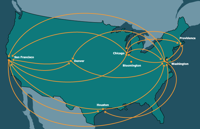
22.2.1 Links by Name
type Key = String

data KeyedNode:
  | keyed-node(key :: Key, content, adj :: List<String>)
end

type KNGraph = List<KeyedNode>

type Node = KeyedNode
type Graph = KNGraphkn- stands for “keyed node”.
kn-cities :: Graph = block:
  knWAS = keyed-node("was", "Washington", [list: "chi", "den", "saf", "hou", "pvd"])
  knORD = keyed-node("chi", "Chicago", [list: "was", "saf", "pvd"])
  knBLM = keyed-node("bmg", "Bloomington", [list: ])
  knHOU = keyed-node("hou", "Houston", [list: "was", "saf"])
  knDEN = keyed-node("den", "Denver", [list: "was", "saf"])
  knSFO = keyed-node("saf", "San Francisco", [list: "was", "den", "chi", "hou"])
  knPVD = keyed-node("pvd", "Providence", [list: "was", "chi"])
  [list: knWAS, knORD, knBLM, knHOU, knDEN, knSFO, knPVD]
endfun find-kn(key :: Key, graph :: Graph) -> Node:
matches = for filter(n from graph):
n.key == key
end
matches.first # there had better be exactly one!
endExercise
Convert the comment in the function into an invariant about the datum. Express this invariant as a refinement and add it to the declaration of graphs.
fun kn-neighbors(city :: Key,  graph :: Graph) -> List<Key>:
  city-node = find-kn(city, graph)
  city-node.adj
endcheck:
ns = kn-neighbors("hou", kn-cities)
ns is [list: "was", "saf"]
map(_.content, map(find-kn(_, kn-cities), ns)) is
[list: "Washington", "San Francisco"]
end22.2.2 Links by Indices
In some languages, it is common to use numbers as names. This is
especially useful when numbers can be used to get access to an element
in a constant amount of time (in return for having a bound on the
number of elements that can be accessed). Here, we use a list—
ix- stands for
“indexed”.
data IndexedNode:
  | idxed-node(content, adj :: List<Number>)
end

type IXGraph = List<IndexedNode>

type Node = IndexedNode
type Graph = IXGraphix-cities :: Graph = block:
inWAS = idxed-node("Washington", [list: 1, 4, 5, 3, 6])
inORD = idxed-node("Chicago", [list: 0, 5, 6])
inBLM = idxed-node("Bloomington", [list: ])
inHOU = idxed-node("Houston", [list: 0, 5])
inDEN = idxed-node("Denver", [list: 0, 5])
inSFO = idxed-node("San Francisco", [list: 0, 4, 3])
inPVD = idxed-node("Providence", [list: 0, 1])
[list: inWAS, inORD, inBLM, inHOU, inDEN, inSFO, inPVD]
end0. To find a node:
fun find-ix(idx :: Key, graph :: Graph) -> Node:
  lists.get(graph, idx)
endfun ix-neighbors(city :: Key, graph :: Graph) -> List<Key>:
city-node = find-ix(city, graph)
city-node.adj
endcheck:
ns = ix-neighbors(3, ix-cities)
ns is [list: 0, 5]
map(_.content, map(find-ix(_, ix-cities), ns)) is
[list: "Washington", "San Francisco"]
endSomething deeper is going on here. The keyed nodes have
intrinsic keys: the key is part of the datum itself. Thus, given
just a node, we can determine its key. In contrast, the indexed nodes
represent extrinsic keys: the keys are determined outside the
datum, and in particular by the position in some other data
structure. Given a node and not the entire graph, we cannot know for
what its key is. Even given the entire graph, we can only determine
its key by using identical, which is a rather unsatisfactory
approach to recovering fundamental information. This highlights a
weakness of using extrinsically keyed representations of
information. (In return, extrinsically keyed representations are
easier to reassemble into new collections of data, because there is no
danger of keys clashing: there are no intrinsic keys to clash.)
22.2.3 A List of Edges
le- stands for “list of edges”.
data Edge:
  | edge(src :: String, dst :: String)
end

type LEGraph = List<Edge>

type Graph = LEGraphle-cities :: Graph =
[list:
edge("Washington", "Chicago"),
edge("Washington", "Denver"),
edge("Washington", "San Francisco"),
edge("Washington", "Houston"),
edge("Washington", "Providence"),
edge("Chicago", "Washington"),
edge("Chicago", "San Francisco"),
edge("Chicago", "Providence"),
edge("Houston", "Washington"),
edge("Houston", "San Francisco"),
edge("Denver", "Washington"),
edge("Denver", "San Francisco"),
edge("San Francisco", "Washington"),
edge("San Francisco", "Denver"),
edge("San Francisco", "Houston"),
edge("Providence", "Washington"),
edge("Providence", "Chicago") ]fun le-neighbors(city :: Key, graph :: Graph) -> List<Key>:
neighboring-edges = for filter(e from graph):
city == e.src
end
names = for map(e from neighboring-edges): e.dst end
names
endcheck:
le-neighbors("Houston", le-cities) is
[list: "Washington", "San Francisco"]
end22.2.4 Abstracting Representations
We would like a general representation that lets us abstract over the
specific implementations. We will assume that broadly we have
available a notion of Node that has content, a notion of
Keys (whether or not intrinsic), and a way to obtain the
neighbors—
22.3 Measuring Complexity for Graphs
Before we begin to define algorithms over graphs, we should consider how to measure the size of a graph. A graph has two components: its nodes and its edges. Some algorithms are going to focus on nodes (e.g., visiting each of them), while others will focus on edges, and some will care about both. So which do we use as the basis for counting operations: nodes or edges?
No two nodes are connected. Then there are no edges at all.
Every two nodes is connected. Then there are essentially as many edges as the number of pairs of nodes.
Therefore, when we want to speak of the complexity of algorithms over graphs, we have to consider the sizes of both the number of nodes and edges. In a connected graphA graph is connected if, from every node, we can traverse edges to get to every other node., however, there must be at least as many edges as nodes, which means the number of edges dominates the number of nodes. Since we are usually processing connected graphs, or connected parts of graphs one at a time, we can bound the number of nodes by the number of edges.
22.4 Reachability
Many uses of graphs need to address reachability: whether we can, using edges in the graph, get from one node to another. For instance, a social network might suggest as contacts all those who are reachable from existing contacts. On the Internet, traffic engineers care about whether packets can get from one machine to another. On the Web, we care about whether all public pages on a site are reachable from the home page. We will study how to compute reachability using our travel graph as a running example.
22.4.1 Simple Recursion
If they are the same, then clearly reachability is trivially satisfied.
If they are not, we have to iterate through the neighbors of the source node and ask whether the destination is reachable from each of those neighbors.
fun reach-1(src :: Key, dst :: Key, g :: Graph) -> Boolean:
  if src == dst:
    true
  else:
    <graph-reach-1-loop>
    loop(neighbors(src, g))
  end
endsrc is:
fun loop(ns):
  cases (List) ns:
    | empty => false
    | link(f, r) =>
      if reach-1(f, dst, g): true else: loop(r) end
  end
endcheck:
reach = reach-1
reach("was", "was", kn-cities) is true
reach("was", "chi", kn-cities) is true
reach("was", "bmg", kn-cities) is false
reach("was", "hou", kn-cities) is true
reach("was", "den", kn-cities) is true
reach("was", "saf", kn-cities) is true
endExercise
Which of the above examples leads to a cycle? Why?
22.4.2 Cleaning up the Loop
Before we continue, let’s try to improve the expression of the
loop. While the nested function above is a perfectly reasonable
definition, we can use Pyret’s for to improve its readability.
fun ormap(fun-body, l):
  cases (List) l:
    | empty => false
    | link(f, r) =>
      if fun-body(f): true else: ormap(fun-body, r) end
  end
endfor ormap(n from neighbors(src, g)):
reach-1(n, dst, g)
end22.4.3 Traversal with Memory
Because we have cyclic data, we have to remember what nodes we’ve already visited and avoid traversing them again. Then, every time we begin traversing a new node, we add it to the set of nodes we’ve already started to visit so that. If we return to that node, because we can assume the graph has not changed in the meanwhile, we know that additional traversals from that node won’t make any difference to the outcome.This property is known as ☛ idempotence.
fun reach-2(src :: Key, dst :: Key, g :: Graph, visited :: List<Key>) -> Boolean:
  if visited.member(src):
    false
  else if src == dst:
    true
  else:
    new-visited = link(src, visited)
    for ormap(n from neighbors(src, g)):
      reach-2(n, dst, g, new-visited)
    end
  end
endfalse. (There may still be other parts of the graph to explore,
which other recursive calls will do.)Exercise
Does it matter if the first two conditions were swapped, i.e., the beginning ofreach-2began withif src == dst: true else if visited.member(src): false? Explain concretely with examples.
Exercise
We repeatedly talk about remembering the nodes that we have begun to visit, not the ones we’ve finished visiting. Does this distinction matter? How?
22.4.4 A Better Interface
reach-2 shows, we may have a better
implementation, but we’ve changed the function’s interface; now it has
a needless extra argument, which is not only a nuisance but might also
result in errors if we accidentally misuse it. Therefore, we should
clean up our definition by moving the core code to an internal
function:
fun reach-3(s :: Key, d :: Key, g :: Graph) -> Boolean:
  fun reacher(src :: Key, dst :: Key, visited :: List<Key>) -> Boolean:
    if visited.member(src):
      false
    else if src == dst:
      true
    else:
      new-visited = link(src, visited)
      for ormap(n from neighbors(src, g)):
        reacher(n, dst, new-visited)
      end
    end
  end
  reacher(s, d, empty)
endExercise
Does this really gives us a correct implementation? In particular, does this address the problem that the
sizefunction above addressed? Create a test case that demonstrates the problem, and then fix it.
22.5 Depth- and Breadth-First Traversals
It is conventional for computer science texts to call these depth- and breadth-first search. However, searching is just a specific purpose; traversal is a general task that can be used for many purposes.
The reachability algorithm we have seen above has a special property. At every node it visits, there is usually a set of adjacent nodes at which it can continue the traversal. It has at least two choices: it can either visit each immediate neighbor first, then visit all of the neighbors’ neighbors; or it can choose a neighbor, recur, and visit the next immediate neighbor only after that visit is done. The former is known as breadth-first traversal, while the latter is depth-first traversal.
The algorithm we have designed uses a depth-first strategy: inside <graph-reach-1-loop>, we recur on the first element of the list of neighbors before we visit the second neighbor, and so on. The alternative would be to have a data structure into which we insert all the neighbors, then pull out an element at a time such that we first visit all the neighbors before their neighbors, and so on. This naturally corresponds to a queue [An Example: Queues from Lists].
Exercise
Using a queue, implement breadth-first traversal.
If we correctly check to ensure we don’t re-visit nodes, then both
breadth- and depth-first traversal will properly visit the entire
reachable graph without repetition (and hence not get into an infinite
loop). Each one traverses from a node only once, from which it
considers every single edge. Thus, if a graph has \(N\) nodes and
\(E\) edges, then a lower-bound on the complexity of traversal is
\(O([N, E \rightarrow N + E])\). We must also consider the cost of checking whether we
have already visited a node before (which is a set membership problem,
which we address elsewhere: Making Sets Grow on Trees). Finally, we have to
consider the cost of maintaining the data structure that keeps track
of our traversal. In the case of depth-first traversal,
recursion—
This would suggest that depth-first traversal is always better than breadth-first traversal. However, breadth-first traversal has one very important and valuable property. Starting from a node \(N\), when it visits a node \(P\), count the number of edges taken to get to \(P\). Breadth-first traversal guarantees that there cannot have been a shorter path to \(P\): that is, it finds a shortest path to \(P\).
Exercise
Why “a” rather than “the” shortest path?
Do Now!
Prove that breadth-first traversal finds a shortest path.
22.6 Graphs With Weighted Edges
Consider a transportation graph: we are usually interested not only in whether we can get from one place to another, but also in what it “costs” (where we may have many different cost measures: money, distance, time, units of carbon dioxide, etc.). On the Internet, we might care about the ☛ latency or ☛ bandwidth over a link. Even in a social network, we might like to describe the degree of closeness of a friend. In short, in many graphs we are interested not only in the direction of an edge but also in some abstract numeric measure, which we call its weight.
In the rest of this study, we will assume that our graph edges have weights. This does not invalidate what we’ve studied so far: if a node is reachable in an unweighted graph, it remains reachable in a weighted one. But the operations we are going to study below only make sense in a weighted graph.We can, however, always treat an unweighted graph as a weighted one by giving every edge the same, constant, positive weight (say one).
Exercise
When treating an unweighted graph as a weighted one, why do we care that every edge be given a positive weight?
Exercise
Revise the graph data definitions to account for edge weights.
Exercise
Weights are not the only kind of data we might record about edges. For instance, if the nodes in a graph represent people, the edges might be labeled with their relationship (“mother”, “friend”, etc.). What other kinds of data can you imagine recording for edges?
22.7 Shortest (or Lightest) Paths
Imagine planning a trip: it’s natural that you might want to get to your destination in the least time, or for the least money, or some other criterion that involves minimizing the sum of edge weights. This is known as computing the shortest path.
We should immediately clarify an unfortunate terminological
confusion. What we really want to compute is the lightest
path—
Exercise
Construct a graph and select a pair of nodes in it such that the shortest path from one to the other is not the lightest one, and vice versa.
We have already seen [Depth- and Breadth-First Traversals] that breadth-first search constructs shortest paths in unweighted graphs. These correspond to lightest paths when there are no weights (or, equivalently, all weights are identical and positive). Now we have to generalize this to the case where the edges have weights.
w :: Key -> Numberw :: Key -> Option<Number>some value it will be the weight; otherwise the
weight will be none.Now let’s think about this inductively. What do we know initially?
Well, certainly that the source node is at a distance of zero from
itself (that must be the lightest path, because we can’t get any
lighter). This gives us a (trivial) set of nodes for which we already
know the lightest weight. Our goal is to grow this set of
nodes—
Inductively, at each step we have the set of all nodes for which we know the lightest path (initially this is just the source node, but it does mean this set is never empty, which will matter in what we say next). Now consider all the edges adjacent to this set of nodes that lead to nodes for which we don’t already know the lightest path. Choose a node, \(q\), that minimizes the total weight of the path to it. We claim that this will in fact be the lightest path to that node.
If this claim is true, then we are done. That’s because we would now add \(q\) to the set of nodes whose lightest weights we now know, and repeat the process of finding lightest outgoing edges from there. This process has thus added one more node. At some point we will find that there are no edges that lead outside the known set, at which point we can terminate.
It stands to reason that terminating at this point is safe: it corresponds to having computed the reachable set. The only thing left is to demonstrate that this greedy algorithm yields a lightest path to each node.
We will prove this by contradiction. Suppose we have the path \(s \rightarrow d\) from source \(s\) to node \(d\), as found by the algorithm above, but assume also that we have a different path that is actually lighter. At every node, when we added a node along the \(s \rightarrow d\) path, the algorithm would have added a lighter path if it existed. The fact that it did not falsifies our claim that a lighter path exists (there could be a different path of the same weight; this would be permitted by the algorithm, but it also doesn’t contradict our claim). Therefore the algorithm does indeed find the lightest path.
What remains is to determine a data structure that enables this algorithm. At every node, we want to know the least weight from the set of nodes for which we know the least weight to all their neighbors. We could achieve this by sorting, but this is overkill: we don’t actually need a total ordering on all these weights, only the lightest one. A heap see Wikipedia gives us this.
Exercise
What if we allowed edges of weight zero? What would change in the above algorithm?
Exercise
What if we allowed edges of negative weight? What would change in the above algorithm?
For your reference, this algorithm is known as Dijkstra’s Algorithm.
22.8 Moravian Spanning Trees
At the turn of the milennium, the US National Academy of Engineering surveyed its members to determine the “Greatest Engineering Achievements of the 20th Century”. The list contained the usual suspects: electronics, computers, the Internet, and so on. But a perhaps surprising idea topped the list: (rural) electrification.Read more about it on their site.
22.8.1 The Problem
To understand the history of national electrical grids, it helps to go back to Moravia in the 1920s. Like many parts of the world, it was beginning to realize the benefits of electricity and intended to spread it around the region. A Moravian academia named Otakar Borůvka heard about the problem, and in a remarkable effort, described the problem abstractly, so that it could be understood without reference to Moravia or electrical networks. He modeled it as a problem about graphs.
The electrical network must reach all the towns intended to be covered by it. In graph terms, the solution must be spanning, meaning it must visit every node in the graph.
Redundancy is a valuable property in any network: that way, if one set of links goes down, there might be another way to get a payload to its destination. When starting out, however, redundancy may be too expensive, especially if it comes at the cost of not giving someone a payload at all. Thus, the initial solution was best set up without loops or even redundant paths. In graph terms, the solution had to be a tree.
Finally, the goal was to solve this problem for the least cost possible. In graph terms, the graph would be weighted, and the solution had to be a minimum.
22.8.2 A Greedy Solution
Begin with a solution consisting of a single node, chosen arbitrarily. For the graph consisting of this one node, this solution is clearly a minimum, spanning, and a tree.
Of all the edges incident on nodes in the solution that connect to a node not already in the solution, pick the edge with the least weight.Note that we consider only the incident edges, not their weight added to the weight of the node to which they are incident.
Add this edge to the solution. The claim is that for the new solution will be a tree (by construction), spanning (also by construction), and a minimum. The minimality follows by an argument similar to that used for Dijkstra’s Algorithm.
Jarník had the misfortune of publishing this work in Czech in 1930, and it went largely ignored. It was rediscovered by others, most notably by R.C. Prim in 1957, and is now generally known as Prim’s Algorithm, though calling it Jarník’s Algorithm would attribute credit in the right place.
Implementing this algorithm is pretty easy. At each point, we need to know the lightest edge incident on the current solution tree. Finding the lightest edge takes time linear in the number of these edges, but the very lightest one may create a cycle. We therefore need to efficiently check for whether adding an edge would create a cycle, a problem we will return to multiple times [Checking Component Connectedness]. Assuming we can do that effectively, we then want to add the lightest edge and iterate. Even given an efficient solution for checking cyclicity, this would seem to require an operation linear in the number of edges for each node. With better representations we can improve on this complexity, but let’s look at other ideas first.
22.8.3 Another Greedy Solution
Recall that Jarník presented his algorithm in 1930, when computers didn’t exist, and Prim his in 1957, when they were very much in their infancy. Programming computers to track heaps was a non-trivial problem, and many algorithms were implemented by hand, where keeping track of a complex data structure without making errors was harder still. There was need for a solution that was required less manual bookkeeping (literally speaking).
In 1956, Joseph Kruskal presented such a solution. His idea was elegantly simple. The Jarník algorithm suffers from the problem that each time the tree grows, we have to revise the content of the heap, which is already a messy structure to track. Kruskal noted the following.
To obtain a minimum solution, surely we want to include one of the edges of least weight in the graph. Because if not, we can take an otherwise minimal solution, add this edge, and remove one other edge; the graph would still be just as connected, but the overall weight would be no more and, if the removed edge were heavier, would be less.Note the careful wording: there may be many edges of the same least weight, so adding one of them may remove another, and therefore not produce a lighter tree; but the key point is that it certainly will not produce a heavier one. By the same argument we can add the next lightest edge, and the next lightest, and so on. The only time we cannot add the next lightest edge is when it would create a cycle (that problem again!).
Therefore, Kruskal’s algorithm is utterly straightforward. We first
sort all the edges, ordered by ascending weight. We then take each
edge in ascending weight order and add it to the solution provided it
will not create a cycle. When we have thus processed all the edges, we
will have a solution that is a tree (by construction), spanning
(because every connected vertex must be the endpoint of some edge),
and of minimum weight (by the argument above). The complexity is that
of sorting (which is \([e \rightarrow e \log e]\) where \(e\) is the
size of the edge set. We then iterate over each element in \(e\),
which takes time linear in the size of that set—
22.8.4 A Third Solution
Both the Jarník and Kruskal solutions have one flaw: they require a
centralized data structure (the priority heap, or the sorted list) to
incrementally build the solution. As parallel computers became
available, and graph problems grew large, computer scientists looked
for solutions that could be implemented more efficiently in
parallel—
In 1965, M. Sollin constructed an algorithm that met these needs beautifully. In this algorithm, instead of constructing a single solution, we grow multiple solution components (potentially in parallel if we so wish). Each node starts out as a solution component (as it was at the first step of Jarník’s Algorithm). Each node considers the edges incident to it, and picks the lightest one that connects to a different component (that problem again!). If such an edge can be found, the edge becomes part of the solution, and the two components combine to become a single component. The entire process repeats.
Because every node begins as part of the solution, this algorithm naturally spans. Because it checks for cycles and avoids them, it naturally forms a tree.Note that avoiding cycles yields a DAG and is not automatically guaranteed to yield a tree. We have been a bit lax about this difference throughout this section. Finally, minimality follows through similar reasoning as we used in the case of Jarník’s Algorithm, which we have essentially run in parallel, once from each node, until the parallel solution components join up to produce a global solution.
Of course, maintaining the data for this algorithm by hand is a nightmare. Therefore, it would be no surprise that this algorithm was coined in the digital age. The real surprise, therefore, is that it was not: it was originally created by Otakar Borůvka himself.
pinpointed the real problem lying underneath the electrification problem so it could be viewed in a context-independent way,
created a descriptive language of graph theory to define it precisely, and
even solved the problem in addition to defining it.
As you might have guessed by now, this problem is indeed called the MST in other textbooks, but “M” stands not for Moravia but for “Minimum”. But given Borůvka’s forgotten place in history, we prefer the more whimsical name.
22.8.5 Checking Component Connectedness
As we’ve seen, we need to be able to efficiently tell whether two
nodes are in the same component. One way to do this is to conduct a
depth-first traversal (or breadth-first traversal) starting from the
first node and checking whether we ever visit the second one. (Using
one of these traversal strategies ensures that we terminate in the
presence of loops.) Unfortunately, this takes a linear amount of time
(in the size of the graph) for every pair of nodes—
It is helpful to reduce this problem from graph connectivity to a more general one: of disjoint-set structure (colloquially known as union-find for reasons that will soon be clear). If we think of each connected component as a set, then we’re asking whether two nodes are in the same set. But casting it as a set membership problem makes it applicable in several other applications as well.
The setup is as follows. For arbitrary values, we want the ability to
think of them as elements in a set.
We are interested in two operations. One is obviously union,
which merges two sets into one. The other would seem to be something
like is-in-same-set that takes two elements and determines
whether they’re in the same set. Over time, however, it has proven
useful to instead define the operator find that, given an
element, “names” the set (more on this in a moment) that the element
belongs to. To check whether two elements are in the same set, we then
have to get the “set name” for each element, and check whether these
names are the same. This certainly sounds more roundabout, but this
means we have a primitive that may be useful in other contexts, and
from which we can easily implement is-in-same-set.
none case of parent):
data Element<T>:
  | elt(val :: T, parent :: Option<Element>)
endfun is-same-element(e1, e2): e1.val <=> e2.val endDo Now!
Why do we check only the value parts?
fynd because find is already defined to mean
something else in Pyret. If you don’t like the misspelling, you’re
welcome to use a longer name like find-root.
fun is-in-same-set(e1 :: Element, e2 :: Element, s :: Sets)
    -> Boolean:
  s1 = fynd(e1, s)
  s2 = fynd(e2, s)
  identical(s1, s2)
endSets is the list of all elements:
type Sets = List<Element>is-same-element; when we do, we check the
element’s parent field. If it is none, that means this
very element names its set; this can happen either because the element
is a singleton set (we’ll initialize all elements with none),
or it’s the name for some larger set. Either way, we’re
done. Otherwise, we have to recursively find the parent:
fun fynd(e :: Element, s :: Sets) -> Element:
  cases (List) s:
    | empty => raise("fynd: shouldn't have gotten here")
    | link(f, r) =>
      if is-same-element(f, e):
        cases (Option) f.parent:
          | none => f
          | some(p) => fynd(p, s)
        end
      else:
        fynd(e, r)
      end
  end
end
Exercise
Why is there a recursive call in the nested
cases?
union. For this, we find the
representative elements of the two sets we’re trying to union; if they
are the same, then the two sets are already in a union; otherwise, we
have to update the data structure:
fun union(e1 :: Element, e2 :: Element, s :: Sets) -> Sets:
  s1 = fynd(e1, s)
  s2 = fynd(e2, s)
  if identical(s1, s2):
    s
  else:
    update-set-with(s, s1, s2)
  end
endfun update-set-with(s :: Sets, child :: Element, parent :: Element)
-> Sets:
cases (List) s:
| empty => raise("update: shouldn't have gotten here")
| link(f, r) =>
if is-same-element(f, child):
link(elt(f.val, some(parent)), r)
else:
link(f, update-set-with(r, child, parent))
end
end
endcheck:
s0 = map(elt(_, none), [list: 0, 1, 2, 3, 4, 5, 6, 7])
s1 = union(get(s0, 0), get(s0, 2), s0)
s2 = union(get(s1, 0), get(s1, 3), s1)
s3 = union(get(s2, 3), get(s2, 5), s2)
print(s3)
is-same-element(fynd(get(s0, 0), s3), fynd(get(s0, 5), s3)) is true
is-same-element(fynd(get(s0, 2), s3), fynd(get(s0, 5), s3)) is true
is-same-element(fynd(get(s0, 3), s3), fynd(get(s0, 5), s3)) is true
is-same-element(fynd(get(s0, 5), s3), fynd(get(s0, 5), s3)) is true
is-same-element(fynd(get(s0, 7), s3), fynd(get(s0, 7), s3)) is true
endFirst, because we are performing functional updates, the value of the
parentreference keeps “changing”, but these changes are not visible to older copies of the “same” value. An element from different stages of unioning has different parent references, even though it is arguably the same element throughout. This is a place where functional programming hurts.Relatedly, the performance of this implementation is quite bad.
fyndrecursively traverses parents to find the set’s name, but the elements traversed are not updated to record this new name. We certainly could update them by reconstructing the set afresh each time, but that complicates the implementation and, as we will soon see, we can do much better.
Exercise
Is it? Consider constructing
unions that are not quite so skewed as above, and see whether you get the results you expect.
The bottom line is that pure functional programming is not a great fit with this problem. We need a better implementation strategy: Disjoint Sets Redux.